EVA as a management tool / Evanomics.com

Helsinki School of Economics and Business Administration
Department of Accounting and Finance

Economic Value Added as a management tool

Esa Mäkeläinen
E-mail: www.evanomics.com
9.2.1998

Table of contents
1 Introduction *
1.1 The objective and motivation of the study *
1.2 The structure of the study *
1.3 Terminology *
1.4 Case-companies and applied conversions *
2 Economic Value Added and its characteristics *
2.1 The main theory behind EVA *
2.1.1 The background of EVA *
2.1.2 Market Value Added defined *
2.2 A review of EVA as performance measure and as a yardstick of wealth creation * 2.2.1 The discrepancy in accounting rate of return (ROI) and EVA *
2.2.2 Some evidence on the correlation between EVA and share prices *
2.2.3 Evidence on EVA in management bonus plans *
2.3 EVA as a performance measure in corporate world * 2.3.1 Implications of EVA in corporate control *
2.3.2 The main problems with EVA in measuring operating performance *
2.3.3 How to improve EVA *
2.3.4 EVA and allocation of capital *
2.3.5 EVA vs. traditional performance measures *
2.3.6 EVA vs. other Value-based measures *
3 EVA in Group-level controlling *
3.1 A rational definition of EVA in business unit management *
3.1.1 Capital, NOPAT and Rate of return *
3.1.2 Taxes in EVA-formula *
3.1.3 Average cost of capital *
3.1.4 The essence of defining the capital costs accurately *
3.2 EVA in Bonus systems * 3.2.1 Arguments for using EVA in bonus systems *
3.2.2 Characteristics of feasible EVA-based bonus system *
3.2.3 The impacts of EVA’s imperfections to bonus system *
3.2.4 Possible EVA-based bonus plans *
3.3 Implementing EVA control inside organization *
4 EVA in case-SBU *
5 Summary and conclusions *
6 Literature references: *

Introduction

Investors are currently demanding Shareholder value more strongly than ever. In the1980s, shareholder activism reached unforeseen levels with the companies in the United States (Bacidore et al. 1997). Thereafter also investors in Europe have increased the pressure on companies to maximize shareholder value. Even in Finland the so-called Shareholder value –approach has gained grounds. This is due to e.g. abolishing the restrictions on foreign stock ownership. Foreign investors emphasize and demand focus on Shareholder value -issues. (Löyttyniemi 1996)
The financial theory has since long suggested that every company’s ultimate aim is to maximize the wealth of its shareholders. That should be natural since shareholders own the company and as rational investors expect good long-term yield on their investment. In the past, this ultimate aim has however been often partly ignored or at least misunderstood. This can be seen e.g. from measurement systems. Metrics like Return on investment and Earnings per share are used as the most important performance measures and even as a bonus base in a large number of companies, although they do not theoretically correlate with the Shareholder value creation very well. Against this background it is no wonder that so-called Value based measures have received a lot of attention in the recent years. These new performance metrics seek to measure the periodic performance in terms of change in value. Maximizing value means the same as maximizing long-term yield on shareholders’ investment.
Currently the most popular Value based measure is Economic Value Added, EVA™. There has been a vivid debate for and against EVA in academic and management literature. Unfortunately most EVA advocates and adapters have not acknowledged or discussed the faults of EVA, while they have praised the concept as a management tool. On the other hand most criticism against EVA has kept to fairly insignificant topics from the viewpoint of corporate control. There are currently very few articles dealing objectively with EVA’s strengths and weaknesses as a management tool.

The objective and motivation of the study

This study seeks to clarify the concept of EVA especially from the viewpoint of business unit controlling. The objective of the study is twofold. Firstly, the study describes the theory and characteristics of EVA. This gives the framework to discuss the main objective: How companies should use EVA considering both its favorable and unfavorable features? In this context, the study also offers some recommendations of how EVA should be used as a management tool. The study tries to bring together the relevant theoretical issues and controlling practice. The topics discussed are essential and current in the case-group as well as in many other companies implementing EVA-approach in their organizations.

The structure of the study

The study consists of three main chapters. The first discusses the general theory behind EVA. This chapter presents the background and basic theory of EVA as well as main findings about EVA in financial literature. The chapter explains also in general what EVA has to give to corporate world. The second chapter focuses on the use of EVA in group-level controlling. It discusses how EVA could be defined in controlling and reporting, how it can be used in bonus systems and what are the problems faced in implementing EVA. The third and final main chapter deals with EVA more practically inside the case SBU. The chapter presents with numerical example the calculation of EVA and the impacts of a few different calculation methods. Chapter also illustrates one possible way to allocate the capital costs in the case SBU.

Terminology

Shareholder value = Shareholder value is being used as a overall term covering various aspects in thinking that promotes the interests of shareholders. Normally the term also means a company’s value to its shareholders i.e. market capitalization.
Shareholder value approach = Shareholder value approach refers to the focus of organization and management on acting within the interests of shareholders. Hence it means focus on maximizing the wealth of shareholders (creating shareholder value).
Value based measures = Value based measures are new performance measures that originate from the shareholder value approach. They seek to measure the periodic performance in terms of shareholder value created (or destroyed).

Case-companies and applied conversions

The subject will be discussed from both the viewpoint of the case-group and the case-SBU (Strategic business unit). The case-SBU is a unit of the case-group. From the reader’s point of view it is completely irrelevant which real companies this study deals with. Therefore the group and the parent company will be called Group A or (parent) Company A. The Group and the parent company have the same name also in reality. The SBU (daughter company) will be called Company B or SBU B. Company B has been a kind of EVA-pilot in the case-group, since it has used EVA in reporting and bonus systems from the beginning of this year (1997). This naturally influences the whole study. Some problems are discussed in the light of these early experiences.
All of the figures in this study have been conversed linearly, so that meaning of the figures and the respective relations between the figures are still unchanged even though they do not relate to any real numbers.

Economic Value Added and its characteristics

This chapter presents the main theory about EVA and shows some empirical findings around the concept in financial literature. The last section 2.3 tries to present what the theory of EVA means in practice for companies.

The main theory behind EVA

EVA measures whether the operating profit is enough compared to the total costs of capital employed. Stewart defined EVA (1990, p.137) as Net operating profit after taxes (NOPAT) subtracted with a capital charge:
EVA = NOPAT – CAPITAL COST Û
EVA = NOPAT – COST OF CAPITAL x CAPITAL employed (1)
Or equivalently, if rate or return is defined as NOPAT/CAPITAL, this turns into a perhaps more revealing formula:
EVA = (RATE OF RETURN – COST OF CAPITAL) x CAPITAL (2)
Where:

Rate of return = Nopat/Capital

Capital = Total balance sheet minus non-interest bearing debt in the beginning of the year

Cost of capital = Cost of Equity x Proportion of equity from capital + Cost of debt x Proportion of debt from capital x (1-tax rate). Cost of capital or Weighted average cost of capital (WACC) is the average cost of both equity capital and interest bearing debt. Cost of equity capital is the opportunity return from an investment with same risk as the company has. Cost of equity is usually defined with Capital asset pricing model (CAPM). The estimation of cost of debt is naturally more straightforward, since its cost is explicit. Cost of debt includes also the tax shield due to tax allowance on interest expenses. This derivation of equity cost and WACC is explained later in detail with chapter 4.2 (Company B’s EVA).

If ROI is defined as above (after taxes) then EVA can be presented with familiar terms to be:
EVA = (ROI – WACC) x CAPITAL EMPLOYED (3)
The idea behind EVA is that shareholders must earn a return that compensates the risk taken. In other words equity capital has to earn at least same return as similarly risky investments at equity markets. If that is not the case, then there is no real profit made and actually the company operates at a loss from the viewpoint of shareholders. On the other hand if EVA is zero, this should be treated as a sufficient achievement because the shareholders have earned a return that compensates the risk. This approach - using average risk-adjusted market return as a minimum requirement - is justified since that average return is easily obtained from diversified long-term investments on stock markets. Average long-term stock market return reflects the average return that the public companies generate from their operations.
EVA is based on the common accounting based items like interest bearing debt, equity capital and net operating profit. It differs from the traditional measures mainly by including the cost of equity. Mathematically EVA gives exactly the same results in valuations as Discounted cash flow (DCF) or Net present value (NPV) (Stewart 1990, p.3 and Käppi 1996), which are long since widely acknowledged as theoretically best analysis tools from the Shareholders perspective (Brealey & Mayers 1991 p.73-75). These both measures include the opportunity cost of equity, they take into account the time value of money and they do not suffer from any kind of accounting distortions. However, NPV and DCF do not suit in performance evaluation because they are based exclusively on cash flows. EVA in turn suits particularly well in performance measuring. Yet, it should be emphasized that the equivalence with EVA and NPV/DCF holds only in special circumstances (in valuations) and thus this equivalence does not have anything to do with performance measurement. This peculiar characteristic of EVA is explained later in detail.

The background of EVA

EVA is not a new discovery. An accounting performance measure called residual income is defined to be operating profit subtracted with capital charge. EVA is thus one variation of residual income with adjustments to how one calculates income and capital. According to Wallace (1997, p.1) one of the earliest to mention the residual income concept was Alfred Marshall in 1890. Marshall defined economic profit as total net gains less the interest on invested capital at the current rate. According to Dodd & Chen (1996, p.27) the idea of residual income appeared first in accounting theory literature early in this century by e.g. Church in 1917 and by Scovell in 1924 and appeared in management accounting literature in the 1960s. Also Finnish academics and financial press discussed the concept as early as in the 1970s. It was defined as a good way to complement ROI-control (Virtanen 1975, p.111). Knowing this background many academics have been wondering about the big publicity and praise that has surrounded EVA in the recent years. The EVA-concept is often called Economic Profit (EP) in order to avoid problems caused by the trademarking. On the other hand the name "EVA" is so popular and well known that often all residual income concepts are often called EVA although they do not include even the main elements defined by Stern Stewart & Co. For example, hardly any of those Finnish companies that have adopted EVA calculate rate of return based on the beginning capital as Stewart has defined it, because average capital is in practice a better estimate of the capital employed. So they do not actually use EVA but other residual income measure. This insignificance detail is ignored later on in order to avoid more serious misconceptions. It is justified to say that the EVA concept Finnish companies are using corresponds virtually the EVA defined by Stern Stewart & Co.
In the 1970s or earlier residual income did not got wide publicity and it did not end up to be the prime performance measure in great deal of companies. However EVA, practically the same concept with a different name, has done it in the recent years. Furthermore the spreading of EVA and other residual income measures does not look to be on a weakening trend. On the contrary the number of companies adopting EVA is increasing rapidly (Nuelle 1996, p.39, Wallace 1997, p.24 and Economist 1997/2). We can only guess why residual income did never gain a popularity of this scale. One of the possible reasons is that Economic value added (EVA) was marketed with a concept of Market value added (MVA) and it did offer a theoretically sound link to market valuations. In the times when investors demand focus on Shareholder value issues this was a good bite. Perhaps also pertinent marketing by Stern Stewart & Co. had and has its contribution.

Market Value Added defined

EVA is aimed to be a measure that tells what have happened to the wealth of shareholders. According to this theory, earning a return greater than the cost of capital increases value (of a company), and earning less decreased value. For listed companies Stewart defined another measure that assesses if the company has created shareholder value. If the total market value of a company is more than the amount of capital invested in it, the company has managed to create shareholder value. If the case is opposite, the market value is less than capital invested, the company has destroyed shareholder value. Stewart (1990,153) calls that difference between the company’s market and book value as Market Value Added or MVA™ for short.
MarkeT Value Added =
company’s total Market Value - capital invested
and with simplifying assumption that market and book value of debt are equal, this is the same as:
MarkeT Value Added =
Market Value of Equity - Book Value of Equity (3)
Book value of equity refers to all equity equivalent items like reserves, retained earnings and provisions. In other words, in this context, all the items that are not debt (interest bearing or non-interest bearing) are classified as equity.
Market value added is identical by meaning with the market-to-book -ratio. The difference is only that MVA is an absolute measure and market-to-book -ratio is a relative measure. If MVA is positive that means that market-to-book -ratio is more than one. Negative MVA means market-to-book -ratio less than one.
According to Stewart Market value added tells us how much value company has added to, or subtracted from, its shareholders’ investment. Successful companies add their MVA and thus increase the value of capital invested in the company. Unsuccessful companies decrease the value of the capital originally invested in the company. Whether a company succeeds in creating MVA (increasing shareholder value) or not, depends on its rate of return. If a company’s rate of return exceeds its cost of capital, the company will sell on the stock markets with premium compared to the original capital (has positive MVA). On the other hand, companies that have rate of return smaller than their cost of capital sell with discount compared to the original capital invested in company. Whether a company has positive or negative MVA depends on the level of rate of return compared to the cost of capital. All this applies also to EVA. Thus positive EVA means also positive MVA and vice versa. Stewart (p. 153) defined in his book the connection between EVA and MVA.
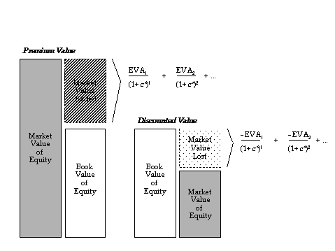
MarkeT Value Added = Present value of all future eva (4)
Market value added is equal to present value of all future EVA. Increasing EVA a company increases its market value added, or in other words increases the difference between company’s value and the amount of capital invested in it.
The relationship with EVA and MVA has its implications on valuation. By arranging the formulas above we find a new definition of the value of company:
Market Value of Equity =
Book Value of Equity + Present value of all future eva (5)
Following figure will illustrate this relationship between EVA and MVA:

Figure 1 Company's market value depends directly on its future EVA.

The phenomenon with rate of return and MVA is in one sense similar to the relationship between the yield and market value of a bond. If the yield of a bond exceeds the current market interest rate (cost of capital) then the bond will sell at a premium (there is positive EVA and so the bond will sell at positive MVA). If the yield of a bond is lower than the current market interest rate then the bond will sell at discount (there is negative EVA and so the bond will sell at negative MVA).
If the net assets or "capital" in the EVA formula (formula 2) reflected the current value of a company’s assets and if the "rate of return" reflected the true return, then there would not be much questioning about the theory between EVA and MVA. After all, nobody questions the above connection between the market value, face value, interest rate and yield of a bond (obviously not since it hold almost perfectly also in practise). But with MVA and EVA things are little bit more complicated. The term "capital" in formula 2 does not reflect the current value of assets, because the capital is based on historical values. Nor does the "rate of return" reflect the true return of the company. All accounting based rate of returns (ROI, RONA, ROCE, ROIC) fail to assess the true or economic return of a firm, because they are based on the historical asset values, which in turn are distorted by inflation and other factors (Villiers 1997, p.287). Stewart defines his rate of return as return on beginning capital and as return after taxes but these adjustments do not affect the problems attached to accounting rate of return. The shortcomings of accounting rate of returns and the current research on the subject are presented in detail in next section (2.2.1.).
The valuation formula of EVA (formula 5) however is always equivalent to Discounted cash flow and Net present value, if EVA is calculated as Stewart presents. Thus the above valuation formula (formula 5) gives always the right estimate of value (same as DCF and NPV) no matter what the original book value of equity is. This holds true even though capital is not an unbiased estimate of current value of assets and rate of return is not an unbiased estimate of the true return. That is because an increase in book value (formula 5) decreases the periodic EVA-figures (and of course a decrease in book value increases EVA-fig.) and these changes cancel each other out. Also this phenomena will be discussed more in next section (2.2.1).

A review of EVA as performance measure and as a yardstick of wealth creation

The discrepancy in accounting rate of return (ROI) and EVA

Every project that a firm undertakes should have positive Net present value (NPV) in order to be acceptable from the shareholders point of view. This means that a project should have internal rate of return bigger than the cost of capital. With practical performance measuring the internal rate of return can not be measured and some accounting rate of return is used instead to estimate the rate of return to capital. Typically this rate of return is some form of return on investment (ROI). Unfortunately any accounting rate of return can not on average produce an accurate estimate of the underlying true rate of return. Following example illustrates this problem, which is more thoroughly and with stronger theoretic background discussed below. The example presents an investment project with initial investment of 1200, duration of 8 years, constant gross profit of 210, IRR of 11% and with no salvage value.

Table A: Example how ROI estimates (both in different years and on average) the return of an investment producing a IRR of 11%.

Year 1 2 3 4 5 6 7 8

Cash flows

Investment -1200

Gross margin 210 210 210 210 210 210 210 210

Total Cash flow -990 210 210 210 210 210 210 210

Depreciation -150 -150 -150 -150 -150 -150 -150 -150

Operating income 60 60 60 60 60 60 60 60

Balance sheet

Beginning assets 1200 1050 900 750 600 450 300 150

Ending assets 1050 900 750 600 450 300 150 0

Accounting returns

ROI (beginning) 5,00 % 5,71 % 6,67 % 8,00 % 10,00 % 13,33 % 20,00 % 40,00 %

ROI (average) 5,33 % 6,15 % 7,27 % 8,89 % 11,43 % 16,00 % 26,67 % 80,00 %

True return and Net present value

IRR 11,0 % 11,0 % 11,0 % 11,0 % 11,0 % 11,0 % 11,0 % 11,0 %

NPV (WACC 10%) 29

Different averages of ROIs Normal average Harmonic mean Geo-metric mean Normal mean weighted with assets

ROI based on beginning capital 13,59 % 8,9 % 10,6 % 8,9 %

ROI based on average capital 20,22 % 10,0 % 13,0 % 10,0 %

Figure 2: How ROI estimates the return of an 8-year-project in different years. The true return or IRR of the project is 11% (shown as a vertical line).

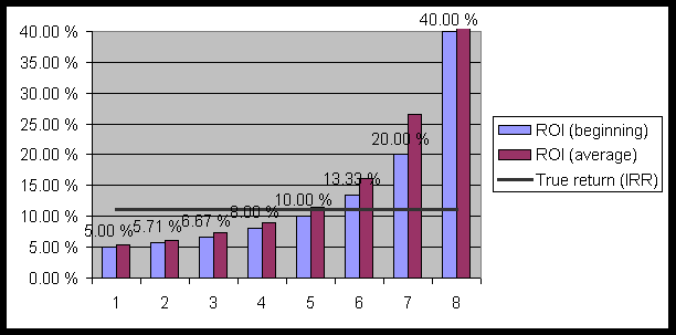
As the above example indicates, ROI is a poor indicator of the true rate of return of the project. The Table A and the Figure 2 illustrate how ROI underestimates the IRR in the beginning and overestimates it in the end on the period. In the remaining study this phenomenon is called wrong periodizing. Besides that ROI periodizes the rate of return wrongly in this example and it also on average fails to estimate the true rate of return of the project. That can be seen from the different averages of ROI in the bottom of the Table A. None of them is the same as IRR. In this case ROI underestimates the true return. In the real life inflation increases the cash flows compared to the initial investment and thus ROI might as well overestimate the true return.
The wrong periodizing is with a real project perhaps even fiercer than in the above example. That is because usually in the real life projects the positive cash flows are generated only some time after the beginning of the period. For example investment in a new plant or machinery starts to generate positive cash flows only after construction and installation phase. It also takes some time to reach the full potential of new machines and it might take some time to establish new product in the markets.
However a company is typically a continuous stream of investments and not a single big investment. Therefore the problem of wrong periodizing of accounting rate of return is with performance measurement not as big a problem as with a single investment. Furthermore, a company has also a big proportion of current assets that reduce the problem of wrong periodizing. That is because there are approximately as much current assets in the beginning as in the end of the investment period. However the wrong periodizing is a problem. Companies can have a big proportion either very old or young assets. It is seldom the case that there are equal proportions of old, young and middle aged assets in a company’s balance sheet. Thus if a company has a lot of new assets, new investments, it its likely to have low ROI although its true rate of return were sufficient. In the opposite case, a company has very little new investments compared to the major investments made in the past. This kind of example can be e.g. a very old paper mill: Since the original investment is depreciated, the assets are very small. Therefore a moderate operating cash flow might produce a very high ROI although the true return for the whole investment period is even lower than the cost of capital. This kind of situation might give the management wrong signals of the true profitability of a business. Thus it might lead to either overinvestments in mature businesses or underinvestments in profitable businesses. Furthermore, on the basis of the above example (Table A and Figure 2), it is easy to see that ceasing investments leads to increase in ROI in the short run.
In addition to wrong periodizing ROI is also otherwise a poor measure of company’s true rate of return. The discrepancy between the accounting rate of return and the true return is well documented in economic literature. Harcourt (1965), Salomon and Laya (1967), Livingston and Salomon (1970), Fischer and McGowan (1983) and Fisher (1984) concluded that the difference between accounting rate of return and the true rate of return is so large that the former can not be used as an indication of the latter (REF De Villiers 1997, p.286-287). The effect of inflation on the discrepancy was addressed by Salomon and Laya (1967), Kay (1976), Van Breda (1981) Kay and Mayer (1986) and De Villiers (1989). They have shown that inflation exacerbates the discrepancy between accounting and true return. (REF De Villiers 1997, p.286-287) Although inflation strengthens the discrepancy, it should be pointed out that accounting rate of return is not, on average, equal to the true rate of return even with no inflation.
Salomon and Laya (1967) studied the accounting rate of return (ARR) and the extent to which it approximates the true return measured with IRR. The IRR of a project can be measured, but because the projects constituting a firm are usually not visible, the true yield of a firm is unknown (Salomon and Laya, 1967, p. 157). The authors therefore studied a theoretical firm made up from projects with a known IRR, and found that the ARR of the firm differs from the IRR of the projects underlying the theoretical firm. The authors also show by means of a numerical simulation that inflation increases the ARR of a firm when IRR is being held at constant. (REF De Villiers 1989, p. 494-495)
De Villiers (1989) studies the relationship between accounting and true rate of return with different asset structures. Typically firms can have three different type of assets: Current assets (inventories and receivables), Depreciable assets (e.g. machinery&equipment and buildings) and Non-depreciable assets (e.g. land and stocks). De Villiers (1989) finds that if a firm had nothing but current assets, ROI (on average) would equal IRR. However, the more a firm has depreciable assets (ceteris paribus), the more ROI overstates IRR. On the other hand the more firm has non-depreciable assets (ceteris paribus) the more ROI understates IRR. In the real world companies have assets of all these three kinds and their relative proportions determine whether ROI underestimates or overestimates IRR (and true rate of return). De Villiers (1989) also presents that even if the assets are valued at their current value (and not at their historical value) there is still some discrepancy between ROI and IRR. In other words when the understatement of asset value (caused by inflation and historical values) is eliminated there is still discrepancy between ROI and IRR that can thereby be ascribed to a deficiency in the accounting profit only. (De Villiers 1989, p.502-503) De Villiers concludes that accounting rates of return of firms with different asset structures are not comparable.
Alongside with inflation rate and asset structure, also the length of investment period affects the discrepancy between ROI and IRR. Other factors being constant, the longer investment period (economic life of assets) the bigger is the discrepancy between ROI and IRR. This is obvious since long investment period gives inflation time to distort asset values. The effect of the project duration to the discrepancy is shown in the article of De Villiers (1997, p.293-294).
Since EVA is calculated from the accounting based numbers and some version of accounting return is used in calculating EVA, it is obvious that all the discrepancies mentioned above affect also EVA. If ROI overstates IRR then EVA also overstates the real shareholder value added. De Villiers (1997) demonstrates with numerical examples how big these distortions can be. He also suggests the use of a modified concept of EVA called adjusted EVA (or AEVA) in order to radically decrease these discrepancies. The adjusted EVA is simple using current value of all assets in calculating the accounting rate of return (ROI). De Villiers pointed out that one should not use market values of equity in calculating EVA as so often is done. Using market value of equity would be circular reasoning and lead to EVA of zero. Instead current value (market value) of individual assets produce much more sound result, but they are admittedly often either very difficult or even impossible to estimate. The use of current value of assets does not however eliminate the discrepancy wholly but it does diminish it to a fraction of original discrepancy.
Storrie & Sinclair (1997) present also that EVA based on historical values can be somewhat misleading. They first demonstrate that the valuation formula of EVA is theoretically exactly the same as the valuation formula of discounted cash flow (DCF) (Proved also by Käppi 1996). After that Storrie & Sinclair also prove mathematically that this equivalence is due to the fact that the book value in EVA valuation formula is irrelevant in determining value. That is because an increase in "book value of equity" (formula 5 below) decreases the periodic EVA-figures ("present value of future EVA") and these changes cancel each other out.

Market value of equity = Book value of equity + present value of future EVA (5)
Book value of equity affects the periodic EVA figures in future via capital costs: If book value of equity is too high then the capital costs in future are also too high and the periodic EVA values too low. These opposite changes in the two terms cancel each other and thus the market value of equity is always the same no matter of the original book value. This is quite simple to demonstrate with an example:
Suppose that a company does an asset revaluation of +100 and thus increases its book value of equity from 500 to 600. The increase in net worth is naturally only an accounting trick and does not affect the market value of company. Let us examine the impact of this trick to above EVA-valuation formula (formula 5). The additional book value of 100 increases periodical capital costs with 100 x WACC (let us assume that this additional book value of 100 is undepreciable, which makes the example easier). If WACC is assumed to be 10%, then the increase in periodic capital costs is 10. How much does this periodic increase in capital costs decrease the present value of EVA? Well, if the additional capital cost decreases periodic EVA by 10 with each year then the whole impact can be calculated as a present value of this 10. The present value of this 10 is 10/0,1 = 100 (The Gordon model: the present value of infinite and constant cash flow: PV= D/r). Hence the decrease in present value of EVA (-100) is with absolute value exactly the same as the increase in book value of equity (+100). Therefore this action does not affect the market value of equity calculated with EVA.
As we can see the decrease in the present value is exactly as big as the increase in book value, so the initial book value does not matter in valuation. More generally proofed:
Change in present value of future EVA = (Change in book value x capital cost)/capital cost = Change in book value (6)
The situation does not change even if the change in book value was depreciable. Then the additional depreciation and additional capital costs correspond together the change in book value.
This is the reason why a measure like EVA based on accounting items can produce theoretically equivalent result with discounted cash flow although we know that accounting based measures and accounting based rate of returns are somewhat distorted. According to Storrie & Sinclair (1997):
The mathematical equivalence is achieved because the EVA formula is a modified version of a standard DCF formula within a mathematical construct in which all of the adjustments in the EVA formula to the DCF must result net to zero. The result of this construct is that it does not matter what beginning capital base is used in an EVA valuation – the result value will always be identical.
EVA valuation formula gives the true value of a firm no matter how the accounting is done. This is achieved with combining income statement and balance sheet. Double entry bookkeeping ensures that everything must add up and that accounting numbers have some connection with economically meaningful variables such as cash flow and dividends. This discipline applies however only when profit is computed on a "comprehensive income" basis:
Opening book value of equity
+ Accounting profit
- Dividends (less new issues of equity)
= Closing book value of equity
For this relationship to hold, profit must include all valuation adjustments affecting the balance sheet. In some countries it is possible to violate against this principle. (O’Hanlon & Peasnell, 1996)
Although in valuation the capital base does not matter, it might cause harm in performance measurement because the periodic values of EVA are distorted. This distortion can be abolished almost entirely by using current value of assets in calculating capital costs, but again this might be time-consuming and difficult and it might not pass a prudent cost benefit analysis in practical business situation (Dodd&Chen 1996, p.28). It should also be noted that in practice EVA seldom corresponds DCF, because any adjustment made to EVA abolishes the mathematical equivalence (Storrie&Sinclair 1997, p.5).
Also the original EVA consulting company Stern Stewart & Co has noticed and reacted to the distortions in periodic EVA figures. The company recommends that after introducing a simple definition of EVA, the concept can be refined to the degree that makes sense taking into account both the costs and benefits of complicating the model. According to Stern Stewart, two most important ways to decrease accounting distortions are introducing a modified depreciation schedule or imposing a level capital charge throughout the life of the asset. Either of these prevents EVA from increasing simply because an asset is growing older. (Kroll 1997, p.105) The level capital charge means probably that the sum of depreciation plus capital cost of an asset is the same every year during the economic life of the asset in question. Normally the depreciation is the same every year (straight-line depreciation) and thus the sum of depreciation and capital costs is big in early years and diminishes towards the end.

Some evidence on the correlation between EVA and share prices

As already presented (in chapter 2.1.2.) according to the EVA-theory the market value of a company is its book value plus the current value of future EVA (formula 5). This strict relationship between EVA and the market value of a company suggests that EVA drives the market values of shares. This relationship between EVA and MVA has been studied in the recent years in many studies with many methods - and with different results.
Stewart (1990, p.215 - 218) has first studied this relationship with market data of 618 U.S. companies. Stewart presents the results in his book "The quest for value". He states that EVA and MVA correspond each other in reality quite well among US companies (the data was from late 1980’s). Only the relationship between negative EVA and negative MVA does not hold very well. According to Stewart, this is because the potential of liquidation, recovery, recapitalization, or takeover sets a floor on a company’s market value (Stewart p.217). For example with companies which have a lot of fixed assets this is quite easy to understand. Market value will always reflect the value of assets even though the company has very low or negative rate of return (and so theoretically it should sell a lot below book value). That is because the company can always be liquidated; the owners have an option to liquidate the assets if the return looks week also in the future. On the other hand markets do not believe that the weak returns can go on forever. Markets are expecting a chance, an improvement, in the long run. If EVA is positive, the relationship is more direct. Then the market valuation happens on the basis of return and growth potential and not on the basis of liquidation or recovery value. Stewart finds also that MVA and EVA correspond each other best when we talk about changes in EVA and MVA and not the absolute levels. Changes in EVA and MVA are not affected so much by accounting distortions and inflation than the absolute values.
Lehn and Makhija (1996) study EVA and MVA as performance measures and signals for strategic change. Their data consists of 241 U.S. companies and cover years 1987, 1988, 1992 and 1993. The researchers first find out that both measures correlate positively with stock returns and that the correlation is slightly better than with traditional performance measures like return on assets (ROA), return on equity (ROE) and return on sales (ROS). Additionally they study how companies’ performance, as measured in terms of EVA and MVA, affect on the CEO firings. Finally they examine the relationship between EVA/MVA and corporate focus. Lehn and Makhija find an inverse relation between EVA/MVA and abnormal CEO turnover. They also find that firms with greater focus on their business activities have significantly higher MVA than their less focused counterparts. Lehn and Makhija conclude that their results suggest EVA and MVA to be effective performance measures that contain information about the quality of strategic decisions and serve as signals of strategic change.
Uyemura, Kantor and Pettit (1996) from Stern Stewart & Co present findings on the relationship between EVA and MVA with 100 bank holding companies. They calculate regressions to 5 performance measures including EPS, Net Income, ROE, ROA and EVA. According to their study the correlations between these performance measures and MVA are: EVA 40%, ROA 13%, ROE 10%, Net income 8% and EPS 6%. The data is from the ten-year period 1986 through 1995.
O’Byrne (1996) from Stern Stewart & Co uses capitalized EVA as independent variable in a regression where market value divided by capital is the dependent variable. He finds that the level of EVA explains 31% of the variance in market value, whereas the level of net operating profit after taxes explains only 17%. When looking at changes in EVA and market value O’Byrne finds that changes in EVA explain 55% of variations in changes in market value. Changes in NOPAT explain only 33%.
Milunovich and Tsuei (1996) review the correlations between MVA and several conventional performance measures in the computer industry. They find EVA to correlate somewhat better with MVA than the other measures. R squared is for EVA 0,42, for EPS growth 0,34 and for ROE and EPS 0,29.
Grant (1996) calculates regression statistics between the MVA-to-capital and EVA-to-capital ratios from the data of 983 firms. He finds explanatory levels (R squared) of 32% with statistical significance. Regressing MVA-to-capital and the spread between return and cost of capital reveals R squared of 37%.
Dodd and Chen (1996) study the correlation between stock returns and different profitability measures including EVA, non-adjusted residual income, ROA, EPS and ROE. In their study ROA explained stock returns best with R squared of 24,5%. The R squared for other metrics are: EVA 20,2%, residual income 19,4% and EPS, ROE approximately 5-7%. The writers concluded that firms adopting EVA might as adopt simple residual income concept, while residual income correlates with share prices almost as well as its adjusted version called EVA. The study is based on 566 U.S. companies from 1983-1992.
Biddle. Bowen and Wallace (1996) present evidence on the relative and incremental information content of EVA, residual income, earnings and operating cash flow. According to the abstract of the study, the writers conclude that "residual income and/or EVA add incremental information in some settings, but that, on average, neither dominates earnings as a performance measure".
Telaranta’s study on Finnish Stock markets
The only public study about the correlation of EVA and share prices that has been done on Finnish data is from Tero Telaranta 1997. The study and article based to it concluded that EVA is not any better than traditional performance measures. Many Finnish corporate managers have taken these conclusions very seriously and therefore it is more than justified in this context to examine the study more thoroughly that the studies above.
Telaranta (1997a) study how residual income variables explain movements in market valuations of Finnish companies. The data consist of 42 Finnish industrial companies during 1988 –1995. Only 26 of the companies were listed the whole period and 16 were listed for shorter period. During the research period both the aggregate Market value added and the non-weighted average return on stock among the sample companies are negative. That is because the whole Finnish economy and stock markets experienced a severe recession in the middle of research period around the turn of the decade (1990). Telaranta (1997a) use various different methods in assessing the ability of different measures to explain market movements. As dependent variables he use MVA, market-to-book ratio and excess return on stock. As independent variables Telaranta use two versions of economic profit (residual income) and three versions of Eduard-Bell-Ohlson -figure (near residual income) as well as traditional accounting based performance measures like EBITDA, Operating profit, NOPAT, Net earnings and Cash flow. These all measures are regressed also as percentages of sales and as percentage returns on capital, although using residual income variables in that way is not necessarily theoretically sound. The reason for this is probably to get some comparison material for measures like ROI, ROE, Operating profit % and Net earnings %.
Telaranta’s results (1997a) indicate the level of Economic profit (the nearest measure to EVA of all those variables that Telaranta use) to explain 30,7% of the level of Market value added as the next best measure NOPAT explain 30,16%. When talking about changes instead of absolute levels, Economic Profit is the best with R squared of 17,18% whereas Operating profit is the second best with R squared of 16,64%. In several other regressions residual income variables are generally found to be the best measures although with a tiny difference compared to some accounting based variables. In some regressions some accounting based variable is even found to be slightly better than Economic Profit, but these regressions are not very meaningful for one of the following two reasons:

The overall explanatory level with these regressions is far below 5%.

These regressions are on those variables that are all expressed as percentage of sales (e.g. Economic Profit divided with turnover). Economic Profit looses its meaning when expressed as percentage of sales i.e. there is no theory suggesting that variable "Economic Profit/Turnover" should correlate with share prices. Hence there is no meaning attached to the use of Economic Profit with these regressions. Furthermore the explanatory level with these regressions is under 10%.

Telaranta concludes his results to indicate that residual income variables are found to explain the movements in market capitalization with statistical significance. He however founds the explanatory level to be quite low. Telaranta also presents that residual income variables are not found to explain stock returns statistically significantly better than accounting based measures.
Telaranta’s results indicate that Economic Profit is the best variable in the study explaining market movements, but that the difference compared to other measures is insignificant. The difference to accounting based measures is naturally low in terms of statistical significance because the data consists of such a small number of firms. The previous studies on the subject have on average about 15-fold number of companies, so the statistical significance between residual income and accounting based measures is also respectively easier to achieve.
Telaranta also states that the overall explanatory lever is lower than in previous studies. On the other hand Telaranta found an explanatory level of 30% (Economic Profit explains MVA) which settles moderately with other studies (Uyemura et al, EVA 40%), (O’Byrne, EVA 31%), (Milunovich and Tsuei, EVA 42%), (Grant, EVA 32%) and (Dodd and Chen, ROA 24,5%; EVA 20,2%; residual income 19,4%). Telaranta achieve also far lower explanatory levels in regressions with Economic Profit as percentage of sales and Economic Profit as percentage returns on capital. These regressions are however not comparable because they are not based on any theory.
Everyone should also notice the effects of the research period on the results. The aggregate Market value added and the non-weighted average return on stock among the sample companies are negative during the period because of the recession. On the other hand Stewart (1990, p.217) has emphasized that possibility of liquidation sets a floor on company’s MVA. Telaranta’s research period causes thus major bias against EVA. Another unmentioned bias is the use of HEX-index. Especially in the latter half of the period Nokia’s and couple of other companies’ stocks have a very big weight in HEX-index (Nokia currently about 35%). Therefore the impact of one single company is very large in Telaranta's results. If Nokia's stock performance does not correlate very good with Nokia's EVA it would certainly affect the results. Well, Nokia increased its market value to more than 10-fold compared to the beginning of the period and that was of course due to profitable growth prospects (growth in EVA) that the company had ahead. Therefore Nokia's EVA during 1988-1995 hardly explains very much of the change in Nokia's market value during the same period. Nokia´s turnaround from big wealth destroying conglomerate into a big, dynamic wealth creating telecommunications company was firstly seen in share prices and not in profitability measures since investors are staring at future profit prospects (EVA) above the prevailing performance.
Telaranta (1997b) summarize some of his results in Finnish management journal "Talouselämä" in September 1997 and argue that EVA does not create any value added applied as measure or bonus base in companies. Telaranta presents in the article only the results from the regressions where Economic Profit is divided with sales and capital. These regressions do not rank EVA best like the other regressions do. As presented above these regressions are theoretically not sound since any theory does not suggest the variables: "EVA/Turnover" and "EVA/Capital" to correlate with share prices. Also the overall explanatory level of the chosen regressions are very week which also casts doubts on the motives of selection. Why are not the regressions on absolute values selected even though they are theoretically and with explanatory levels far better than those presented in Talouselämä? Telaranta’s article has gained a lot of criticism afterwards (Kurikka 1997 from University of Technology, Torppa&Lumijärvi 1997 from KPMG Management Consulting, Lukka&Tuomela 1997 from Turku School of Economics and Martikainen & Kallunki 1997 from University of Vaasa). Main points of this criticism are:

Periodic EVAs can not explain changes in market values caused by changes in long term EVA (Martikainen&Kallunki 1997 and Torppa&Lumijärvi 1997).

Telaranta can not criticize EVA to be week in corporate control and bonus systems, while he has not studied it (Lukka&Tuomela 1997).

General about the correlation of EVA and share prices
The criticism on Telaranta’s study mentions at least one fundamental hindrance in estimating EVA-theory with stock price correlations: Market values are above all based on expectations about the future cash flows. Changes in the current share prices thus reflect changes in future cash flow and future EVA expectations. Therefore current EVA can never explain current share prices very well. Change in current EVA might imply some change in future EVA and therefore EVA has some explanatory power. On the other hand the change in future EVA is surely visible also in other measures than EVA. Therefore it is understandable that the other measures have almost as much explanatory power and it is also understandable that the explanatory level is quite low with every measure. Still, current research on the subject seems to suggest that EVA has some additional information compared to conventional measures. However EVA should not be viewed as a magic wand, which can explain current share prices with current performance. The power of EVA is elsewhere, in the field of corporate control, and the rest of this study tries to illuminate it. However if EVA is used as Discounted cash flow to estimate current valuations with future EVA estimates it might be quite informative. Perhaps this is why CS First Boston has trained its research staff in EVA analysis, and Goldman Sachs is about to introduce EVA as "a power tool in the analytical tool kit", as global research chief Steve Einhorn from Goldman Sachs put it (Topkis, 1996, p.265).
Of course the relationship between EVA and MVA can and also has to be tested empirically, but the best way to execute these tests is not to correlate periodic EVA and periodic MVA. One way to assess this theory is to calculate MVAs for certain year (-s) and compare them with EVAs from that year on. That is also the way Stewart does in his study. The problem will still be that MVA accounts for all future EVA and not just for EVA of certain period. The shorter period we take the bigger mistake we make in scope. On the other hand the longer period we take, the worse investors’ (EVA) expectations and reality correspond each other. If we compare MVA in 1980 and EVAs in 1981-1990, we assume that investors know in 1980 what is company’s EVA in 1981-1990. In the real life investors do not have crystal ball of ten years. EVA critics should construct their studies to test the EVA theory (MVA is discounted EVA) and not purely periodic correlation with share prices. According to the theory, EVA corresponds MVA and not share prices. That is because simply pouring more money in the company can raise share prices. However EVA and MVA do not rise unless that incremental money earns more than its cost of capital. Therefore e.g. EPS and NOPAT capture much better the share price impacts of NPV negative investments than EVA. Tests should also take into account the liquidation floor of the value of company, because it is part of the EVA-theory Stewart presents. Thirdly and above all, EVA critics should present some logical and theoretical arguments against EVA. There is no sense making hasty conclusions on the grounds of empirical tests if there is no single logical argument along. Investors have always been interested in return and risk and EVA measures these vital things theoretically better than traditional measures.
The distortions in EVA probably affect the correlation between EVA and share prices. This might also be one reason why in spite of its "theoretical superiority", EVA does not correlate with share prices in every study so much better than other accounting based measures like ROI and EPS. The distortions are probably also the main reason why the changes of EVA correlate better with share prices than absolute values. It is also remarkable that those studies excluding all adjustments to EVA (Telaranta 1997, Dodd&Chen, 1996) show least evidence on the correlation.

Evidence on EVA in management bonus plans

Wallace (1997) study the effects of adopting management bonus plans based on residual income measures. The sample in the study consists of forty firms that have some residual income measure, mainly EVA, as bonus base. This sample is compared to sample of same size consisting of similar companies where the bonus is tied to accounting based measures. Wallace tests with various methods the management actions in these sample groups and concludes that "…I interpret the results as being consistent with a residual income-based performance measure providing incentives for managers to act more like owners, thus mitigating the inherent conflict between managers and shareholders." Wallace’s tests support the adage "you get what you measure", with significant increases noted in residual income for the firms adopting residual income based compensation relative to the comparison group. The firms that adopted residual income based compensation outperformed the market over the twenty-four month period by over 4 %-points in cumulative terms.

EVA as a performance measure in corporate world

Implications of EVA in corporate control

In the previous chapters EVA was verified to suffer from the same accounting distortions as any accounting rate of return (e.g. ROI). Therefore EVA might in some occasions give somewhat misleading signals of the true value added to shareholders. In spite of this fact EVA has become a very popular performance measure, perhaps because applying it has some powerful impacts on organizational behavior.
Unlike conventional profitability measures EVA helps the management and also other employees to understand the cost of equity capital. At least in big public companies, which do not have a strong owner, shareholders have often been conceived as a free source of funds. Similarly, business unit managers often seem to think that they have the right to invest all the retained earnings that their business unit has accumulated although the group would have better investment opportunities elsewhere. EVA might change the attitude in this sense because it emphasizes the requirement to earn sufficient return on all capital employed.
Including capital costs in the income statement helps everybody in the organization to see the true costs of capital. Rate of return does not work that way because nobody can explicitly see the costs caused by e.g. inventories, receivables etc. The approaches showing the consequences of invested capital under the line as profit (with ROI) or over the line as cost (with EVA) are totally different. That is why organizations tend to increase their capital turnover after introducing EVA, although they have formerly used ROI that ought to take into account the capital as well. When calculating EVA, the cost of equity (and debt) can be subtracted in the income statement earlier than after the net operating profit. If all the revenues and costs are grouped by functions or by processes, then it is of course practical to allocate the capital costs to these functions or processes. The capital costs can also be allocated directly to products. Part of the capital costs are variable in nature (inventories, trade receivables) and thus they fluctuate according to the sales volume. If the true capital costs were not included fully in product costs, then those cost calculations (for price determination) are misleading. The error is the bigger, the more capital intensive the production is.
At best EVA can be a new approach to view business. Perhaps the biggest benefit of this approach is to get the employees and mangers to think and act like shareholders. It emphasizes that in order to justify investments in the long run they have to produce at least a return that covers the cost of capital. In other case the shareholders would be better off investing elsewhere. This approach includes that the organization tries to operate without lazy or excess capital and it is understood that the ultimate aim of the firm is to create shareholder value by enlarging the product of positive spread (between return and cost of capital) multiplied with the capital employed. The approach creates a new focus on minimizing the capital tied to operations. Firms have so far done a lot in cutting costs but cutting excess capital has been paid less attention. The power of EVA-approach is something that most academic studies about EVA and share price correlation fail to trace. The only way to assess the effects of this approach is to compare two sample groups, other representing firms that use EVA and other firms that do not. Only the study of Wallace (1997) meets this requirement and his study also suggests superior performance with the companies using EVA.

The main problems with EVA in measuring operating performance

As presented earlier EVA and ROI are poor in periodizing the returns of a single investment. They underestimate the return in the beginning and overestimate it in the end of the period. Some growth phase companies or business units have a lot of new investments. Such growth phase companies are likely to have currently negative EVA although their true rate of return would be good and so their true long-term shareholder wealth added (true long-term EVA) would be positive. That is also the reason why EVA is criticized to be a short-term performance measure. Ceasing investments can indeed increase short-term EVA. Some companies have concluded that EVA does not suit them because of their focus on long-term investments that do not occur in a continuous stream. An example is offered by American company GATX (Glasser 1996), which leases transportation equipment and makes fairly long-term investments.
However it should be remembered that the ultimate aim is still to create value for shareholders. Only earning higher rate of return than the cost of capital in the long run can do this. The fact that the required good financial performance is not expected now but only in the future is not a reason to leave out financial measures. Therefore periodic financial performance measures are always important no matter what business field the company operates at. The companies stating that EVA does not suit them because of their long investment horizon are actually presenting that they can manage without measuring the ultimate objective.
This shortsightedness is an inevitable feature with all profitability measures. They all measure current profitability i.e. how current revenues cover current costs. The true return or true EVA of long-term investments can not be measured objectively with any performance measure because future returns can not be measured; they can only be subjectively estimated. If financial performance measures are wanted to maintain as objective measures of current financial performance, they can not include future estimates. With most financial performance measures the only subjective component is the depreciation schedule. Some financial performance measures like CFROI, CVA and DCF have modified depreciation schedules that even out the profitability during the investment period. This of course decreases the objectivity of these measures.
The periodizing problem of financial performance measures has to be managed with focus on long-term. Even though current financial performance is poor, there is no reason to view things with narrow, short-term perspective. This wrong periodizing will even out in the long run, if the investments really are profitable. Furthermore the extent of this problem can be estimated; the average age of company’s asset portfolio can be taken into account in interpreting periodic EVA. It can be expected that companies with a lot of new and thus undepreciable assets have negative EVA in the near future.
The companies that have invested heavily today and expect positive cash flow only in a distant future are extreme examples. For these growth companies - facing profitable long-term opportunities with negative short-term cash flows - EVA is probably not a suitable primary performance measure. The performance of growth companies like some telecommunication operators (heavy investments in infrastructure with very long payoffs) and other high-tech companies is perhaps measured better with market share, change in market share, sales growth etc. That is because the current financial performance of these companies can not be very attractive measured with any metrics.
It certainly holds also more generally that EVA or any other financial performance measure do not in itself provide managers with sufficient information. Financial measures tell us the outcome of many different things. They usually hide the causes of good or bad profitability. The good or bad performance of individual processes is seldom visible in financial performance measures. Some other measures pinpoint the current situation of critical success factors much better. Therefore every company should use many measures in estimating how their plans are going and strategic goals are reached.
The new but famous concept called Balanced Scorecard (Kaplan&Norton 1996) presents that companies should use several different perspectives in measuring performance. The perspectives suggested are (Kaplan&Norton 1996, p.9):

Financial (How should we appear to our shareholders?)

Customer (How should we appear to our customers?)

Internal Business Process (To satisfy our shareholders and customers, what business processes must we excel at?)

Learning and growth (To achieve our vision, how will we sustain our ability to change and improve?)

The relative weight of each group of measures (perspective) depends heavily on the business field and situation of the company. Professors Kaplan and Norton present that in order to fulfill financial objectives set by shareholders, the company should concentrate on besides financial measures also on measures of the other perspectives. If a company has measured customer perspective well and reacted in it with operations (internal business process perspective), the result is often improved financial performance. Financial measures do not often show the reasons but the consequences. Therefore it is utmost important to have also other measures. Sometimes focus on EVA and shareholder value is incorrectly viewed as opposite approach to Balanced Scorecard. On the contrary professors Kaplan and Norton (1996, p. 49) present that EVA is one suitable and widely used financial performance measure for financial perspective. According to Kaplan and Norton (1996) the financial perspective is the critical summary and the main goal. It must not be neither over- nor underemphasized. "A failure to convert improved operational performance in the Scorecard, into improved financial performance should send executives back to their drawing boards to rethink the company’s strategy or its implementation plans." (Kaplan&Norton 1996, p.34). In the end, every strategic plan has to convert into long run profitability in order to be justified.
A good example of the necessity of different measures is provided with the browser and other Internet software producer Netscape. The company did huge losses in its early years but still it was viewed as valuable company because of the expected big positive future cash flows. There would have been no sense in measuring Netscape's current EVA and steering the company on the basis of it. On the other hand company must have some plans about how and when they are going to cash in their lucrative prospects. Enormous growth and customer satisfaction does not comfort the owners if the company can not make money with them. Actually Netscape is currently in a dangerous zone because its sales revenues for 1997 are $533 Million, Operating loss -$132 Million and total shareholders equity $429 Million. If it can not improve its financial performance quickly or raise more capital from shareholders it will go into bankruptcy in less than two years.

The impacts of EVA’s accounting distortions in performance measurement
EVA suffers (as found out in chapter 2.2) also from other distortions than only wrong periodizing. As ROI fails (on average) to estimate the underlying true return, so does the periodic EVA figure fail to estimate (on average) the value added to shareholders, because of the inflation and other factors. Using the current value of assets instead of book values (De Villiers 1997, p.299) can eliminate this problem almost totally. The extent of this problem depends very heavily on the asset structure (how big relative are the proportions of current, depreciable and non-depreciable assets) and on average project duration. Thus the extent and direction of this problem can be estimated. The EVA targets can be adjusted accordingly, although this is not necessary an easy task.
It is however reasonable to admit that this problem is usually so small that no adjustments are necessary. EVA can be and also has been applied successfully in many companies without any special adjustments to capital base (Birchard 1996). This is also the way that companies have calculated their ROI for decades without massive criticism. So far this distortion in ROI has been widely ignored, although the theoretical weakness in using historical values in calculating ROI has been acknowledged e.g. in Finland at least since 1970’s (Virtanen 1975, p.102). This might tell us something about the importance and extent of the effects with this phenomenon. On the other hand it might also tell how difficult these distortions are to bypass.

How to improve EVA

There are countless individual operational things that create shareholder value and increase EVA. Often EVA does not directly help in finding ways to improve operational efficiency except when improving capital turnover. Nor does EVA help directly in finding strategic advantages that enable a company to earn abnormal returns and thus create shareholder value. It is however often helpful to understand the basic ways in which EVA and thus the wealth of shareholders can be improved. Increasing EVA falls always into one of the following three categories:

Rate of return increases with the existing capital base. It means that more operating profits are generated without tying any more capital in the business.

Additional capital is invested in business earning more than the cost of capital. (Making NPV positive investments.)

Capital is withdrawn or liquidated from businesses that fail to earn return greater than the cost of capital.

The first method includes all the countless ways to improve operating efficiency or increase revenues. Of course increasing rate of return with current operations and new investments (that is categories 1 and 2) are often linked; in order to improve the efficiency of ongoing operations, companies often do investments which enhance also the return on current capital base.
The fact that the wealth of shareholders increase with investments returning more that the cost of capital (category 2) is probably known in organizations if they also use some kind of weighted average cost of capital (WACC) and Net present value (NPV) methodology in investment calculations. This rule is actually completely same as accepting only NPV-positive investments.
The third category, withdrawing capital, is probably not so widely understood and applied as the previous ones. It is however also very important to realize that shareholder value can also be increased if capital is withdrawn from businesses earning less than the cost of capital. Even if an operation has positive net income, it might pay to withdraw capital from that activity. It is also kind of withdrawal when access inventories and receivables and thus the capital costs caused by them are reduced without corresponding decreases in revenues.
These categories and ways to improve EVA might appear to be quite simple. They are certainly not new ways to improve the position of shareholders. Decreasing cost of capital is not included in this list of methods. That is because it can not normally be done without changing line of business and in that way changing business risk. Changing financial leverage affects WACC only slightly via increased tax shield. The effects of leverage on capital costs are discussed more thoroughly in chapter 3.

EVA and allocation of capital

EVA is a capital allocation tool both inside a company and also with a broader perspective inside the whole economy. EVA sets a minimum acceptable performance level to the rate of return in the long run. This minimum rate of return is based on the average (risk-adjusted) return on the equity markets. The average return is a benchmark that should be reached. If a company can not achieve the average return, then the shareholders would be better off if they allocated their capital to another industries or to another companies.
There are some lines of business where the average return is in the long run very hard to achieve even with competent management and with no competitive disadvantages. That is normally because these business fields are mature, have excess capacity and thus have very fierce competition. Of course every business field has also some companies that can generate high profitability in spite of the tight situation, but the average return on these businesses is low. These kinds of businesses with low average return have been e.g. steel industry, automobile industry, forest industry, some consumer electronics industries (e.g. television manufacturers) etc. The low return with these fields is likely to improve in the course of time, but it must be emphasised that the question is not about normal business cycles but about long-term disequilibrium between supply and demand i.e. overcapacity. This overcapacity leads these fields inevitably to below average returns.
This kind of fields with low expected return can be identified easily with the market valuations. If the Market value added (MVA) is on average negative with companies of a business field it is a sign that markets do not believe the return with this field to be sufficient in the long run. Negative MVA is a sign that markets believe that a company produces negative EVA in the long run as presented in section 2.1.2.
Majority of the companies with the mature businesses does produce a positive cash flow, although the return is below average. That cash flow in turn is partly distributed to owners as dividends and partly invested back in business. These plowback investments earn the same below average return as the old investments and thus they destroy the wealth of shareholders. In order not to do so, these companies should pay out much more of the free cash flow than currently. Generous dividend policy should continue as long as the expected return is below average return of similar risky investments. This same pattern could be applied within the different business units of a company. Only those business units that can earn at least average return - produce positive EVA in the long run - are entitled to expand their operations with investments.
In the real life it is not necessarily easy to classify business lines that offer below average returns in the long run, because almost all industries have low or even negative return at some point of business cycle. Furthermore there are always companies that are able to generate sufficient returns even with otherwise unprofitable fields. Thirdly all old industries do not necessary end up to be unprofitable since overcapacity arises only in special circumstances.
It is often hard for managers to acknowledge that some business lines are less productive than others are on average. There is however some evidence clearly suggesting that some fields are on average less profitable that others. First of all there are some business lines where all publicly traded companies have negative MVAs suggesting that markets are expecting negative long-term EVA for the field in the future. Furthermore markets have clearly shown to reward certain companies that give up their excess equity capital through share repurchases instead of pouring the money back in business. Especially the big American steel and paper manufacturers that have announced about share repurchasing programs have experienced substantial share price increases (already at the moment of announcement). The shareholder value increases are in these cases due to avoiding the possibility to destroy value with unprofitable investments. Shareholders can invest the money through markets and get easily the average market return whereas these companies would hardly have reached it. On the other hand, if highly profitable companies like Microsoft or Nokia announced that they are going to buy back their shares in order to give up excess equity, their share prices would probably not shoot up but down. That is because their share prices are for the most parts based on the profitable growth with NPV and EVA positive investments.
The problem of investing free cash flow back in unprofitable businesses is widely discussed in literature as part of agency problems (e.g. Jensen 1986). Managers of the unprofitable companies are not willing to give up excess capital since they normally want to grow the operations under their control. Therefore owners or group officers should control investments and develop steering or incentive systems that prevent this kind of behaviour with those fields where it can occur. The misuse of free cash flow to unprofitable investments affects directly EVA-figures and thus using EVA as performance measure might decrease this problem. After all EVA is aimed to be a measure that is consistent with NPV i.e. NPV negative investments decrease EVA and NPV positive investments increase EVA. The study of Wallace (1997, p.15-16) presents empirical evidence that basing compensation on EVA decreases the overinvestments in mature industries. In this context it is important to avoid short run thinking. Negative EVA figures at some period does not always mean that the field is unprofitable in general or that the company does not have any potential for profitable investments. Furthermore some companies might still be able to generate at least average return from the mature industry. In doing so they are able to produce positive EVA and thus justify their own investments.
It is also important to understand that EVA is beneficial capital allocation tool not only for shareholders but also for the economy in general. EVA is a metric measuring if the capital is in efficient use considered the return and risk. Positive EVA is a sign that the capital is in efficient use considered the risk involved in business. On the other hand capital productivity is one factor affecting the whole economy and GDP growth. We have in our economy a certain capital stock and it produces a certain GDP a year. The more productive our capital is the bigger GDP we have. Struggling to reach positive EVA is thus not only good for shareholders, but it benefits the economy and people also in more broad perspective. In practice this beneficial capital allocation might mean that excess capital is moved from forest and steel industry to telecommunication and software industry and it thereafter enables rapid development with these fields and drives down the consumer prices quickly. An overdrawing example: If we had no functioning capital markets then capital could not move from one industry to another. Old industries would keep their capital and invest all the return back in business. We would therefore perhaps pay currently a couple of percent less for our paper and steel but we would still pay 15 000 FIM for a 1 kg mobile phone and 100 000 FIM for a PC with 286-processor…

EVA vs. traditional performance measures

Conceptually, EVA is superior to accounting profits as a measure of value creation because it recognizes the cost of capital and, hence, the riskiness of a firm’s operations (Lehn & Makhija 1996, p.34). Furthermore EVA is constructed so that maximizing it can be set as a target. Traditional measures do not work that way. Maximizing any accounting profit or accounting rate of return leads to an undesired outcome. Following paragraphs seek to clarify the benefits of EVA compared to conventional performance measures.
EVA, NPV vs. IRR, ROI
Return on capital is very common and relatively good performance measure. Different companies calculate this return with different formulas and call it also with different names like Return on investment (ROI), Return on invested capital (ROIC), Return on capital employed (ROCE), Return on net assets (RONA), Return on assets (ROA) etc. The main shortcoming with all these rates of return is in all cases that maximizing rate of return does not necessarily maximize the return to shareholders. Following simple example will clarify this statement:
Suppose a group with two subsidiaries. For both subsidiaries and so for the whole group the cost of capital is 10%. The group names maximizing ROI as target. The other subsidiary has ROI of 15% and the other ROI of 8%. Both subsidiaries begin to struggle for the common target and try to maximize their own ROI. The better daughter company rejects all the projects that produce a return below their current 15% although there would be some projects with return (IRR) 12% - 13%. The other affiliate, in turn, accepts all the projects with return above 8%. For a reason or another (e.g. overheated competition) it does not find very good projects, but the returns of its projects lie somewhere near 9%.
Let us suppose that both subsidiaries manage to increase their ROI. With the better subsidiary ROI increases from 15% to 16% and with the not-so-good subsidiary ROI increases from 8% to 8,5%. The company’s target, increasing ROI, is achieved but what about the shareholder value? It is obvious that all the projects of the not-so-good subsidiary decrease shareholder value, because the cost of capital is more than rate of return (and so the shareholders money would have been better off with alternative investments e.g. in the markets). But the actions of the better subsidiary are neither optimal for shareholders. Of course shareholders will benefit from the good (return over 15%) projects but also all 12%-13% (actually all above 10% = cost of capital) projects should have been accepted even though they decrease current ROI. These projects still create and increase shareholder value.
As the above example demonstrates operations should not be guided with the goal to maximize the rate of return. As a relative measure and without the risk component ROI fails to steer operations correctly. Therefore capital can be misallocated on the basis of ROI. First of all ROI ignores the definite requirement that the rate of return should be at least as high as the cost of capital. Secondly ROI does not recognize that shareholders’ wealth is not maximized when the rate of return is maximized. Shareholders want the firm to maximize the absolute return above the cost of capital and not to maximize percentages. Companies should not ignore projects yielding more than the cost of capital just because the return happens to be less than their current return. Cost of capital is much more important hurdle rate than the company's current rate of return.
Observing rate of return and making decisions based on it alone is similar to assessing products on the "gross margin on sales" -percentage. The product with the biggest "gross margin on sales" -percentage is not necessary the most profitable product. The product profitability depends also on the product volume. In the same way bare high rate of return should not be used as a measure of a company's performance. Also the magnitude of operations i.e. the amount of capital that produces that return is important. High return is a lot easier to achieve with tiny amount of capital than with large amount of capital. Almost any highly profitable company can increase its rate of return if it decreases its size or overlooks some good projects, which produce a return under the current rate of return.
The difference between EVA and ROI is actually exactly the same as with NPV (Net present value) and IRR (Internal rate of return). IRR is a good way to assess investment possibilities, but we ought not to prefer one investment project to the other according to their IRR. Assume two good and exclusive investment projects, project 1 and project 2. Project 1 has lower IRR but is much bigger in scope (bigger initial investment and bigger cash flows and bigger NPV). Project 1 (the project offering lower IRR) is better for shareholders even though it has lower IRR. That is because it provides bigger absolute return than project 2. The reason is exactly same as with ROI: maximizing rate of return percentage does not matter. What matters is the absolute amount of shareholders’ wealth added.
In the corporate control it is worth remembering that EVA and NPV go hand in hand as also ROI and IRR. The formers tell us the impacts to shareholders wealth and the latters tell us the rate of return. There is no reason to abandon ROI and IRR. They are very good and illustrative measures that tell us about the rate of returns. IRR can always be used along with NPV in investment calculations and ROI can always be used along with EVA in company performance. However, we should never aim to maximize IRR and ROI and we should never base decisions on these two metrics. IRR and ROI provide us additional information, although all decisions could be done without them. Maximizing rate of returns (IRR, ROI) does not matter, when the goal is to maximize the returns to shareholders. EVA and NPV should be in the commanding role in corporate control and ROI & IRR should have the role of giving additional information.

Return on equity (ROE)
ROE suffers from the same shortcomings as ROI. Risk component is not included and hence there is no comparison. The level of ROE does not tell the owners if company is creating shareholders wealth or destroying it. With ROE this shortcoming is however much more severe than with ROI, because simply increasing leverage can increase ROE. As we all know, decreasing solvency does not always make shareholders’ position better because of the increased (financial) risk. As ROI and IRR, return on equity (ROE) is also an informative measure but it should not guide the operations.
Earnings and earnings per share (EPS)
EPS is raised simply by investing more capital in business. If the additional capital is equity (cash flow) then the EPS will rise if the rate of return of the invested capital is just positive. If the additional capital is debt then the EPS will rise if the rate of return of the invested capital is just above the cost of debt. In reality the invested capital is a mix of debt and equity and the EPS will rise if the rate of return of that additional capital invested is somewhere between cost of debt and zero. Therefore EPS is completely inappropriate measure of corporate performance and still it is very common yardstick and even a common bonus base. (No wonder shareholders are not too fond of management bonuses.) EPS and earnings can be increased simply by pouring more money into business even though the return on that money would be entirely unacceptable from the viewpoint of owners. EPS, earnings and earnings/EPS growth should therefore be abandoned as performance measures.

EVA vs. other Value-based measures

Besides EVA there are plenty of other Value-based or Shareholder value measures. They are created by consulting industry and/or by academics. Consults are all forced to use their particular acronym of their particular concept although it would not differ very much of the competitors’ measure. Thus the range of these different acronyms is wide. Following mentions only a few of them.
Cash flow return on investment (CFROI) is the product of Boston Consulting Group (BCG) and HOLT Value Associates. It is the long-term internal rate of return defined almost as common IRR. CFROI is determined by converting profitability data into gross cash flow and using real gross assets as an implied investment. CFROI is calculated in two steps: First inflation-adjusted cash flows available to all capital owners in the firm are measured and they are compared with the inflation-adjusted gross investment made by the capital owners. After that the ratio of gross cash flow to gross investment is translated into an internal rate of return by recognizing the finite economic life of depreciating assets and the residual value of non-depreciating assets such as land and working capital (Myers 1996, p.46).
Cash Value Added (CVA) is very similar to EVA except that it includes only cash items. Furthermore it keeps the capital costs constant over certain investment period. CVA is the difference between Operating Cash Flow (OCF) and Operating Cash Flow Demand (OCFD). OCF is the sum of Earnings before Depreciation, Interest and Tax (EBDIT, adjusted for non-cash charges), working capital movement and non-strategic investments. OCFD represents the capital costs. It is the average capital cost per year (in absolute terms) that meets the investors’ financial requirements. OCFD is constant over the investment period. (Ottoson & Weissenrieder, 1996)
Shareholder value Added (SVA) is a creation of Dr. Alfred Rappaport and LEK/Alcar Consulting Group. It origins from the Discounted Cash Flow model and has gained publicity and established position, although is far less used than EVA or CFROI. The idea of SVA is probably roughly the same as Rappaport has presented in his book "Creating Shareholder Value" (1986). That is to discount estimated future cash flows to present and hence continuously calculate the value of the firm. Measuring the current performance is based on comparing these cash flow estimates and period’s real cash flow (Rappaport 1986, p.183). The exact SVA concept is unfortunately documented poorly in public sources.
Adjusted Economic Value Added (AEVA) and Refined Economic Value Added (REVA) are both slightly modified versions of basic EVA and also both created by academics. Adjusted Economic Value Added uses current value of assets instead of book values (De Villiers 1997, p.299). Refined Economic Value Added uses the market value of the firm in the beginning of the period instead of book value (Bacidore et al 1997, p.15).
Unlike EVA many of these other Shareholder value measures are based more on cash flows than EVA. Therefore they do not normally suffer from the same imperfections as EVA does. Hence the rate of return used with these other metrics is usually a good estimate of the underlying true rate of return without any adjustments. The other side of the coin is that these other measures are always quite complicated to calculate. That is the case also with companies that do not need any difficult and time consuming adjustments in calculating sufficiently accurate estimate of their true rate of return. Usually these other value-based measures are also based on more subjective data than EVA is. At least CFROI and CVA defer most of the depreciation into later years in order to achieve smooth return or smooth capital costs. CFROI includes also some salvage value in calculations. These features make the return to divide more evenly between different periods but they also make the performance measures more subjective. That is because part of the future profit is sort of brought into the present. The question is ultimately weather it is better to have a long-term subjective measure or short-term objective measure.
EVA is the most widely used Value-Based performance measure (Myers, 1996, p.42) probably just because it happens to be an easier concept compared to the others. In implementing EVA, one of the most important things is to get the people in organizations to commit to EVA and thereby also to understand EVA (Klinkerman 1997). Even as easy concept as EVA seems to be quite hard to communicate down the organization. That is why complicated measures do not work very well.
Some Value-Based measures have been found to correlate better with share prices than EVA. For example (Dodd & Chen 1996, p.26) find that Cash Flow Return on investment (CFROI) explains share price movements better than EVA. Of course EVA can also be modified in order to avoid some accounting distortions and to correlate better with share prices, but then we have almost as complicated measure as CFROI. The best possible correlation with share prices is not however the main point, especially when the differences in correlations are quite small and also disputable. All the shareholder value metrics are said to be identical to discounted free cash flow -method, so it is no wonder that some prestigious people say that you can relate the results of these metrics "to the fourth decimal points" (Mayers, 1996, p.45-46 and Storrie&Sinclair 1997, p. 5). With the complicated shareholder wealth -measures it is not always the toughest part to communicate these to people, but to calculate these in day-to-day operations. E.g. CFROI calls for taking into account the effects of inflation to asset values and this in turn takes time and resources, in other words: it takes money. Hence it can perhaps in many occasions be stated that the other metrics do not pass a prudent cost-benefit analysis; the additional costs with implementing them instead of EVA are often more than the incremental information achieved with them.

EVA in Group-level controlling

This chapter discusses how EVA should be defined and used in Group-level controlling of operations. First, it is examined in detail how EVA should be defined in order to balance easiness, theoretical correctness and right steering. Thereafter the chapter deals with arguments for and characteristics of EVA bonus systems. Finally the chapter discusses things that are vital in implementing phase of EVA controlling.

A rational definition of EVA in business unit management

The most important reason for making EVA-concept simpler is to facilitate the learning process of operating people. There are plenty of adjustments that make EVA theoretically and/or practically a better measure or a better guideline in assessment of different units. The question is whether it is worth to do these adjustments or not. Every adjustment increases the complexity of the concept although some of them might be technically fairly easy to execute. When the organization has first adopted the basic concept well, it might be good to slightly modify the concept later on.
Avoiding additional costs in drawing the routine reports is also an important reason to simplify the concept. Stewart (1993, p.8) suggests plenty of adjustments to the basic residual income concept in order to avoid some accounting distortions. These adjustments include e.g. changes in depreciation schedule, inflation adjustments, capitalization of R&D and other strategic investments, currency translation etc. As Stewart admits, it is not wise to do all of these adjustments because of the marginal effects with some fields. Many of these adjustments cost something by increasing the workload in reporting. The problem whether to make some individual adjustment to EVA figures or not, can be approached e.g. by answering the following five questions: Will the operating managers understand the change? Will it influence their decisions? How big difference does it make with this company? Can the necessary data be obtained? How much does it cost?
There can also be other reasons to deviate from the theoretically correct way of calculating EVA than to only simplify the concept. For example, it might be for the SBU-managers difficult to realize that equity is costly capital. They might also have an approach that since they have earned the equity in their balance sheet, they also have the right to use it in their own investments. In this kind of situation, it might be useful - at first, in the early years of implementing EVA - to emphasize the cost of equity capital even with the ways that are not theoretically correct. An example of this kind of procedure is given later in the section 3.1.3. "Average cost of capital".
The degree of complexity in EVA can depend on the use of EVA and also on a business unit’s accounting systems resources to make the adjustments needed. If a unit has a new and flexible information system which can easily make few adjustments to EVA then there is naturally no need not to do them. However, there are possibly a lot of units where the accounting systems are not very sophisticated nor very flexible and for those units there is a strong need to make EVA as simple as possible to prevent extra workload for internal reporting staff. The cost and benefits of information should be considered unit by unit or more accurately system by system.

We should perhaps start seeking the practical definition of EVA by examining the individual terms that EVA consists of. In Chapter 2.1.2 EVA was defined with formula 2 to be as:
EVA = (Rate of return-Cost of capital) x Capital =
(NOPAT/Capital – Cost of capital) x Capital
Following paragraphs seek to discuss what the individual terms might include in business practice.

Capital, NOPAT and Rate of return

Stewart (1990) defined capital to be total assets subtracted with non-interest bearing liabilities in the beginning of the period (year). Rate of return e.g. ROI is however typically calculated as return on average net assets, because it is a better estimate of the capital employed than the beginning capital (Telaranta 1997, p. 26). Although using average capital seems to be estimate of the capital employed, the method has also its weaknesses. Average assets include part of the return generated during the year. Yet, calculating rate of return should not include return in the capital side (in denominator) but only in the return side (numerator). That is because the people have used to understand and express return in relation to the initial investment and not in relation to investment's value in the end of the period. For example an investment in stock markets that was a year a ago 100 and is now 110 is said to have earned a return of 10% (10/100) and not a return of 9,1% (10/110). Simply excluding the profit from the ending balance sheet in calculating average assets can prevent this error. In practice the reporting happens at least once a month and so the average assets can be calculated as average of individual months instead of average from the beginning and ending balance sheet.
Net operating profit (NOP) is quite straightforward item. Of course it can and should be also adjusted according to the unique characteristics of the company in question, but normally there is no need to that. NOPAT is derived from NOP simply by subtracting calculated taxes from NOP: NOPAT = NOP x (1-Tax rate). These calculated taxes do not correspond the taxes actually paid because e.g. interest on debt decreases real taxes. The tax shield of debt is however taken into account with the capital costs.
Rate of return is NOPAT divided by capital, so both the definitions of capital and NOPAT affect rate of return. As stated in previous chapter, there are some problems in assessing rate of return with accounting book values. The rate of return might be somewhat distorted because of e.g. inflation and it could also be periodized wrongly. Using current value of assets instead of book values can radically reduce the distortions caused by inflation. This is still not necessarily a sound procedure because it is surely much more costly and difficult than using book values. Furthermore the benefits (the changes of EVA-figures into right direction) could be quite small especially if the company has a big proportion of current assets and the economic life of the fixed assets is relatively short.
The problem of wrong periodizing can be remedied with using different depreciation method in internal accounting. Normal straight-line depreciation will tend to underestimate the true internal rate of return in the early years and overestimate it in the later years. Using an economic depreciation schedule, known as the "sinking fund" method, will eliminate this distortion. Under sinking-fund depreciation, an asset is written off in the same way that a banker amortizes the principal on a mortgage. This means that in the early years most of the cash the asset generates is used to provide for the return on capital, and only a small fraction amortizes the capital balance. In the latter years it is the opposite. This schedule records little depreciation early on and more later on, but a steady rate of return and hence EVA is recorded over the life of the asset. Also all other depreciation methods that weight the depreciation more heavily into the later years will reduce the problem of wrong periodizing. However all these methods increase the subjectivity of EVA because they sort of bring some part of future profitability into present. Furthermore they are in most cases unnecessary because with steady capital spending program the periodizing problem is immaterial. (Stewart 1993, p.15-16)

Taxes in EVA-formula

Although taxes are without excess depreciation, increase in reserves etc. about one-fifth of the net income and thus even bigger part of EVA, they are often totally ignored in EVA-control and reporting. E.g. Löyttyniemi (1996b) considers this as a sound approach. This approach can be justified because taxes are not a part of operative activities that should be measured and improved. If the pre-tax EVA is improved, then also the wealth of shareholders is improved. So including taxes in reporting does not change the situation in that sense. It only complicates the concept and calculations. Without taxes the reported income statement is simpler.
However, if taxes are totally ignored, then the minimum acceptable target can not be that pre-tax EVA=0. In order to achieve EVA=0, the pre-tax EVA should naturally be somewhat positive. This is a disadvantage, particularly if EVA is used in bonus systems. The bonuses should in that case be calculated based on the above target EVA. Especially if the bonus is paid for all employees, the zero target would be desirable. Major part of the employees can not comprehend EVA precisely, because they do not know the basic concepts of accounting and finance. On the other hand, it is sufficient for them to know that EVA is somehow (but consistently) calculated net result and if it is positive, it means bonus. A measure with target as zero is also psychologically and conceptually better than some other target level even though EVA would not be used in bonus systems at all.
Taxes in EVA formula according to theory
Normally in calculating EVA taxes are subtracted straight form Net operating profit and the tax shield of debt is taken into account in capital costs:
EVA = net operating profit*(1-tax rate) - WACC*capital
This formula does not take into account that excess depreciation and reserves often decrease the amount of taxes paid in real life. At least taxes can be deferred into a distant future. With continuously growing operations the net reserves increase all the time. The practical tax rate is thus lower than the nominal tax rate.
Adapted way to calculate taxes
It is not very difficult to calculate a good estimation of taxes paid in the period. This can be done by simply subtracting the increase in reserves from Net operating profit before calculating taxes.
EVA = [ Net operating profit - ((Net operating profit – excess dereciation – other increase in reserves)*(tax rate)) ] -WACC*capital
This way the taxes are calculated in the same way as tax authorities do it.
Other method that produces about the same result is to decrease the tax rate somewhat according to the estimated average impact of increased reserves. The tax rate could e.g. be 20% instead of the nominal 28%, if the estimated average impact of reserves would be something like that. This is naturally a method of simplification, but might produce a sufficiently accurate result. Furthermore it would perhaps decrease fluctuations from year to year in tax component.
When the taxes can be deferred into distant future, then considering inflation and the time value of money, it is not of great importance if they have to be paid ever or not. In this case the reserves can be viewed as equity and it is reasonable to deduct the increase in reserves from net operating profit before calculating taxes. However, in some occasions the taxes deferred with reserves have to be paid quite soon if e.g. tax regulation changes or if the company can not do new investments. Then the reserves can not be viewed as equity.
The connection between deferred taxes in income statement and in balance sheet
The question whether or not to subtract increase in reserves from operating profit when calculating taxes and the treatment of deferred taxes in balance sheet should be linked to each other. If reserves are noticed in calculating taxes, then the change in deferred taxes should be treated consistently as profit and the deferred taxes in the balance sheet should also be viewed as equity. This means that deferred taxes should be attached with capital costs. If the reserves are not noticed in calculating taxes then the deferred taxes in balance sheet should consistently be treated as non-interest bearing tax-debt. This means that they should be subtracted from capital as other non-interest bearing liabilities.
It is difficult or impossible to say in advance which of these two methods reflects better the actual situation. However the results of these two methods are not so far away from each other: the other has bigger NOPAT but also bigger capital costs, so the end result (EVA) does not be that much different. From the practical viewpoint: it is easier to ignore reserves in income statement and view deferred taxes as non-interest bearing debt.

Average cost of capital

As explained in chapter 2, the cost of capital is defined as weighted average cost of both equity and debt. The tax shield of debt is noticed with the cost of debt:
Cost of capital = Cost of Equity x (Solvency ratio) + Cost of debt x (1- Solvency ratio) x (1-tax rate)
There are, both in defining the cost of debt and the cost of equity, few different methods and also some variation in results. They are however mainly estimation problems and are of little interest in this context. In other words they do not have anything to do with simplifying the EVA-concept or making it a better functioning controlling tool. Some of these problems are discussed in chapter 4.
The calculation formula of average cost of capital (WACC) includes also the solvency ratio. The solvency ratio usually changes according to business cycles and other factors. Financial theory suggests (Copeland&Weston 1992, p.443-444) that when solvency changes the costs of the equity and debt shift so much that the WACC itself does not change (or it would not change without different tax treatment to debt and equity). When the solvency- or equity-to-debt –ratio decreases, the risk of equity increases. So when the relative proportion of debt from capital increases, the return on equity becomes more volatile and thus also the true cost of equity capital increases. Also the lenders demand higher premiums on debt when the leverage increases. So when solvency ratio decreases both the costs of equity and debt increase and visa versa. The increase in costs of equity and debt cancel out the decrease in WACC caused by bigger relative proportion of cheaper debt capital. Hence the change in WACC is zero (This is illustrated in figure 2 (Alternative 1) on the page after next page.)
The reason why average capital costs do not change according to leverage becomes more intuitive if we think of expected returns. Cost of capital (WACC) reflects the expected return on capital with similar risky businesses because it is an opportunity cost i.e. expected return on similar risky investments. If change in leverage does not affect the expected return of the company (expected ROI) then WACC can not change. Well it is obvious that expected ROI does change according to changes in solvency since solvency does not affect operating profit. Changing only the liabilities-side of the balance sheet, e.g. replacing equity with debt, does not affect the expected return on assets. The expected ROE in turn changes according to changes in leverage. Decreased solvency raises expected ROE because increased financial leverage raises return on equity capital (as well as risk of equity capital). Similarly the expected return on stock market does not depend on how the investors finance their investments. Of course for individual investor, the expected return changes if he uses more financial leverage (debt) with his investment. This affects however only return on his own capital (equity) but not the return for the whole investment. Changing leverage changes always the return and risk of equity and debt capital but it can not influence the underlying expected return of the whole investment. It merely allocates the risk and return in a new manner.
Practical performance reporting with EVA requires a certain procedure how WACC is calculated when solvency ratio changes. The following three examples demonstrate this problem through three different procedures to calculate WACC with different solvency ratios. Examples do not include the tax shield of debt in order to keep things simple.
Suppose that the cost of equity is 15% and the cost of debt is 5%. The target (and normal) solvency ratio of the company is 40%. How WACC can be calculated when solvency ratio is 30% and 50%?
1. Alternative: If we calculate WACC strictly according to financial theory, the costs of equity and debt have to be changed each time the solvency changes. This procedure might be too difficult in practical performance measurement.
2. Alternative: We can calculate WACC each time with the actual solvency ratio and with the same estimated costs of equity and debt. Then WACC changes always according to solvency ratio and thus the result is not in line with financial theory.
3. Alternative: We can calculate WACC each time with the target solvency ratio no matter what the actual solvency is. This procedure produces a result in line with financial theory and additionally it is quite simple.
The following figures will clarify these three procedures.

Figure 3 Alternative 1: WACC is calculated according to financial theory: costs of equity and debt change but WACC remains the same when solvency changes.

Figure 4 Alternative 2: WACC is calculated with actual solvency and fixed costs of debt and equity. WACC thus changes according to solvency. This procedure contradicts with financial theory.

Figure 5 Alternative 3: WACC is calculated with target solvency. WACC remains the same although solvency changes.

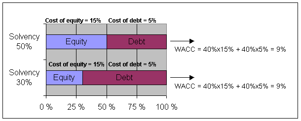
As presented earlier the alternatives 1 and 3 are in line with financial theory: WACC can not be decreased simply by replacing expensive equity capital with cheap debt capital, because solvency affects also the risk level of both equity and debt capital. Therefore alternative 2 (using actual solvency and fixed debt and equity costs) contradicts with the financial theory and seems to be out question. Alternative 1 (changing costs of equity and debt) is best in line with financial theory, but it requires that equity and debt costs should be scaled according to the prevailing solvency ratio. In practice it is therefore too complicated and time-consuming. Alternative 3 (WACC calculated with target solvency ratio) appears to be the best alternative since it is both simple and in accordance with the theory for essential parts. This method does not recognize that costs of equity and debt increase with leverage but on the other hand usually only the average cost of capital (WACC) is of importance. Academics and other experts like Stewart (1990, p.85-89), Löyttyniemi (1996) and Rappaport (1986, p.56) strongly recommend the use of target solvency in calculating WACC and EVA.
Optimal capital structure
The above examples ignored the different tax treatment of debt and equity and some other details. In reality the increased tax shield from debt decreases WACC somewhat when leverage increases. Therefore increasing leverage might decrease WACC slightly. On the other hand if leverage increases too much then the increased probability of bankruptcy and the costs attached to it increase WACC (Copeland&Weston 1992, p.498-499). These bankruptcy costs increase rapidly when solvency decreases from its already low level. Therefore low solvency levels are avoided although mathematically low solvency levels are as good as high since increased return should compensate the increased risk. Correspondingly bankruptcy costs increase at very moderate rate when the solvency decreases from high level. So it does not have very big difference with bankruptcy costs if company's solvency is 90% or 50%. However this would mean a some kind of change in WACC since it affects the tax shield from debt financing. Therefore very high solvency levels are avoided. Although no completely satisfactory financial theory has yet been found to explain the existence of optimal capital structure, casual empiricism suggests that firms behave as though it does exist (Copeland&Weston 1992, p.536). The changes in WACC are nevertheless quite small if the solvency changes moderately and near its optimal level. If e.g. the solvency ratio of an industrial company changes between 40% - 50% it probably has very small impacts on average cost of capital. That is because only changes in tax shield and changes in expected bankruptcy costs affect WACC and their effects are to the opposite directions. This optimal capital structure does change from one business field to another. E.g. real estate companies have on average very low solvency, normal industrial companies have moderate solvency and rapidly growing high-tech companies have high solvency. These different solvency levels reflect the differences in operational risk levels. E.g. real estate companies have very smooth operational cash flow (rents) so they tolerate more financial risk without too high bankruptcy costs. This should be remembered also with business unit controlling. The SBUs with low operational risk might have more financial leverage, lower solvency, than other SBUs.
The calculating of WACC (and EVA) in business controlling should take into account that there is some kind of optimal capital structure. Hence it is not desirable that the solvency ratios of SBUs would differ from it very radically. E.g. if solvency ratio is a SBU is very high, then the tax shield of debt is unused and shareholders will suffer. Furthermore high solvency ratio means besides low risk also low return on equity. However shareholders usually want high return from their investments and tolerate the higher risk level - otherwise they would have invested in bonds instead of in equity /stock market. SBU managers in turn prefer high solvency to low solvency because it is easily to operate with high solvency. High solvency enables the company to do the investments easily without asking for equity capital from parent company. Furthermore high solvency gives more discretion since operational cash flow does not go to fixed interest payments. The companies with high solvency are often referred as companies with "strong balance sheet" or as "healthy" companies. Already these expressions reveal that high solvency is a favorable thing.
If EVA reporting and bonus systems are based on fixed WACC (like example 3 on the previous pages) then EVA does not decrease no matter what the solvency ratio is. In this kind of situation SBU mangers will maintain high solvency and they are not willing to give up excess equity. Group management can of course always force the SBUs to decrease their solvency, but it is quite undesirable situation and leads to lengthy discussions of the "right" solvency level in business units. Better solution would be a controlling or incentive system that steers to optimal (target) solvency. This controlling system can not define WACC as it is in the reality. First of all it is very difficult or impossible to develop a formula that would define the right WACC at each solvency level and secondly this formula would be difficult to use and utmost difficult to communicate throughout organization. Therefore we have to resort to some kind of simplifying procedure. One possible solution would of course be to alter the alternative 3, which calculates WACC with target solvency ratio and fixed costs of equity and debt. WACC could e.g. be raised with 0,5 percentage points or more every time when solvency rises 5 percentage points from its target figure.
Another possible solution might be to turn back to the "incorrect" alternative 2 which calculates WACC with actual solvency and fixed cost of equity and debt. This procedure could be complemented with some sanctions if the solvency falls too low. This kind of system ensures that SBUs give up their excess equity and they would also understand better that equity is costly capital. This procedure includes however one major steering failure.
A steering failure in using actual solvency ratio
The weighted average cost of capital (WACC) should be a factor steering all the capital expenditures and investments. All the investments producing a return above WACC (NPV positive investments) should be executed and all the investments producing a return below WACC should be rejected. In practice this vital condition does not come true if the EVA control uses actual instead of target solvency ratio in calculating WACC. This is because the high solvency ratio enables the company to make quite big investments solely with debt capital. In order to increase EVA, these investments have only to produce a return more than the cost of capital.

EXAMPLE of steering failure when WACC is defined with fixed costs of equity and debt and with actual solvency ratio (alternative 3)
Let us assume that the cost of debt is 5%, the cost of equity 15%, solvency ratio 50% and the beginning capital 100 (equity 50, debt 50). So the current WACC is 10% = 50%*5% + 50%*15%. Let the current return on investment be 11% (operating profit 11). Thus EVA is (ROI - WACC)*CAPITAL = (11%-10%)*100 = 1
The company faces an investment, which requires 25 of capital and offers a return of 6%. The current solvency ratio allows the whole investment to be financed with debt. If the investment were executed, the new capital base would be 125 (equity 50, debt 75). The new operating profit is 11 + 6%*25 = 12,5 and thus return on investment is 10%. WACC would in this new situation be somewhat lower: 0,4*15+0,6*5% = 9% (leverage would change and it would affect WACC). Thus the new EVA would be: (ROI - WACC)*CAPITAL = (10%-9%)*125 = 1,25
When using the actual solvency ratio, EVA might increase with investments producing less than WACC as the above example demonstrates. The increase in EVA is due to mixing operating and financing decisions. The capital resource affects EVA calculated with actual solvency. EVA is simply operating profit minus capital costs and if the investment is financed solely with debt, then the capital costs will only increase with the additional cost of debt. This pattern enables that EVA of a SBU and thus also the management bonuses might increase with accepting investment projects producing less than WACC. This holds only with short-term and with excess solvency. In the long run the company has to use debt and equity with target proportions and with already low solvency it can not solely stick to debt financing. However, the problem must not be underestimated because sometimes people tend to operate in short-term focus and SBUs face often the situation of excess solvency. Reserves and accumulated excess depreciation increase solvency although the net profit of a SBU was divided out as group contribution or dividends.

The essence of defining the capital costs accurately

Historically the ROI-targets are set for SBUs according to their current performance level. If the current performance is good then the ROI-target is also high and visa versa. The board of directors in parent company probably wants to include this kind of pattern also in EVA controlling. This method, defining capital costs according to current performance level and not according to the estimated opportunity cost of capital, is however against the principles of EVA. As presented earlier, the whole meaning with EVA is in establishing a capital cost based on risk-adjusted opportunity cost and that way assuring that the capital is in efficient use.
If the capital costs are set too low, it automatically allows the inefficiency of capital. With too high capital costs the SBUs will ignore some value creating investment opportunities (assuming that the incentive system is efficient). Assume that the cost of capital is set to be 16% and the true opportunity cost of capital is 13%. The SBU will ignore all the investment opportunities producing return between 13% and 16% although they all would improve the position of shareholders. The capital flows to parent company, which is unable to produce a return above 13%. Furthermore, normally most investment possibilities offer a return near the capital costs because we operate in a competitive world. So in this case investments which produce 14% are far more common than investments producing 17%.
With ROI-control the high capital costs are grounded with maintaining current high discipline. If the hurdle rate is decreased, this discipline and the current high profitability are likely to decline. This might be worse than ignoring some good investment opportunities. With EVA approach things are however different. Imposing capital costs well below current rate of return does not leave possibilities to decline current good profitability without decreasing EVA. That is because EVA is the absolute amount of capital the company generates above the capital cost. With EVA control the capital costs should be estimated as objectively as possible. If and when the company wants to set challenging targets they ought to introduce them as high EVA targets, not as high capital costs. There will always be business units with high profitability or with EVA figures biased upwards because of depreciated assets. The EVA targets for those business units should of course be far above zero.
Neither the distortions nor wrong periodizing of EVA should be taken into account in setting the capital costs. That is mainly because the cost of capital is used in estimating investment opportunities with NPV calculations and in this context there are no distortions. Hence modified WACC would cause harm with investment calculations. The distortions in performance measurement can be taken into account in EVA figures, if the company is able to estimate their impact. With steady capital spending program and common asset structure these distortions are usually immaterial.

EVA in Bonus systems

As discussed earlier EVA might be somewhat distorted because of inflation or periodized unevenly inside different years because of flat depreciation schedules. Furthermore it has been presented that these imperfections are exactly the same as problems with accounting rate of return (commonly ROI). If ROI were an accurate estimate of the true underlying return of an enterprise, then EVA would also be an accurate estimate of the excess return to shareholders in absolute terms. In the normal cases, i.e. with relatively stable investment schedule, normal asset structure and reasonable investment horizon ROI can be sufficiently accurate estimate of the true rate of return. Thereby also EVA is accurate enough in estimating the excess return to shareholders in absolute terms. If that is not the case, then ROI and EVA can be adjusted to sufficiently accurate measures with some modifications. Following paragraphs outline first what kind of bonus base EVA would be in the normal case (with no material errors). What the problems of ROI/EVA mean from the viewpoint of bonus systems will be discussed after that.

Arguments for using EVA in bonus systems

If EVA is zero, the shareholders have earned a sufficient rate of return on their capital. Many Finnish companies have earned negative EVA in the long run (Veranen&Junnila 1997). The shareholders of these companies had for sure been better of if the companies have earned positive EVA even though some part of it would have been paid out to company’s managers or employees. The idea of EVA bonuses is that if management can be paid some bonuses, the shareholders have always earned higher return on their capital than they can expect. This kind of bonus system is usually beneficial both to management and the shareholders, because the performance level is likely to rise after introducing EVA bonus system (Wallace 1997). Motivating bonus system normally encourages managers to exceed the normal performance level and even after the payment of the management’s bonuses, the return to shareholders is more than it would have been without the bonus system. With well designed bonus plan, the higher the bonuses that are paid, the better it is for the shareholders. EVA bonus paid is far from a cost to shareholders, because it is often a share in the discretionary value created.
Objective target level
With EVA bonus system the target performance level is very objective. Bonus can be paid e.g. according to some percentage of positive EVA or according to some percentage of improved (positive) EVA. Traditionally bonuses are often subjective, because they are based on the negotiated budgets. The managers negotiating their budgets in turn have incentive to sandbag i.e. to underestimate their potential performance level. That is because revealing the real potential would mean smaller bonus. With objective and unlimited bonus level, the SBU managers have an incentive to maximize performance and value instead of sandbagging their potential and wasting time and effort in managing earnings and the expectations of corporate office. The following citations describe the benefits of objective bonus system:
"Tying incentive compensation to EVA rather than to budget helped streamline the SPX budgeting and planning processes. "No more fussing around in the fall for months, messing around with a huge planning documents and worrying about sandbagging and things like that. It is gone," says Chuck Bowman, director of financial planning and analysis." (Kroll1997, p.109)
"...Instead of having budgets drive bonuses, the bonus system ought to drive the budgets."(Stewart 1990, p. 243)
Agency problems: spending free cash flow
EVA bonus systems are also good in decreasing agency problems. Management of a subsidiary wants usually to invest in their business as much as headquarters allows. Not many SBU management teams conclude voluntarily that they do not have any enough good investment projects and thus it is better to give the period’s free cash flow out as dividends. Even if there would not be enough good investment projects, the subsidiaries would like to keep the excess capital in their balance sheet as liquid assets (or invest it in not-so-good projects). With powerful (enough motivating and rewarding) EVA-based bonus system the management is aimed to avoid this kind of behavior. That is because all capital producing a return less than WACC decreases their bonuses. If the incentives are tied to the change of EVA, excess capital in current assets or overinvestments in mature businesses can do a lot of harm to bonuses. Wallace (1997, p.15-16) presents strong empirical evidence showing that after introducing residual income based bonus system, managers avoid investments producing less than WACC. It applies also more generally, that because EVA measures the ultimate aim of any company, EVA-based bonus systems unite the interest of group management and shareholders or the interest of group and SBU managers.
Paying managers for performance with EVA-based bonus system
Private entrepreneurs, the managers of their own firm get paid just as they make money. Some successful entrepreneurs get rich and there is no set limit to their income level. Corporate managers can often make huge improvements to the wealth of shareholders since they have large amount of capital under management. However mangers are not paid accordingly i.e. with the line of the shareholder wealth increases. Even a little improvement in the capital efficiency might imply a big improvement in shareholder wealth in absolute measures. Some of this kind of big improvement should be paid out to managers in order to motivate managers to top achievements and in order to pay according to performance. In practice that would mean paying more than currently to good performers and less to bad performers.
A method to link the growth of productivity to payroll with line-workers
EVA might also be suitable to uniting the interests of the management/owners and ordinary employees. There has traditionally been an ever-lasting battle between employees and employers. It has led to the rise of strong trade unions and in some cases fruitless, frustrating and wealth-destroying strikes. The problem is that companies’ profits are likely to increase due productivity growth and employees want always to get their share of the increased profit. The employees do not however exactly know what kind of share they could have. They also feel that they are always underpaid compared to the salaries of management and profits of shareholders. Therefore the demand for wage increases are often oversized. Economists tell that wage increases must not be over the growth of productivity (but that is hard to tell to employees, because even economists do not always agree on the definition of the productivity). So the raises often go over the growth of productivity and make profitability and capital efficiency too low from the viewpoint of owners, which in turn decrease employment. Hence the final sufferers are besides shareholders normally also the employees, no matter of employees’ original intention.
EVA-based bonus system might be a way to pay employees according to the change in productivity. If part of the positive EVA is always handed over to employees they might be able to realize the connection between company’s productivity (profitability) and their own payroll. In the last resort, the customers and the productivity pay the payroll and not the owners. EVA bonuses could also bring some elasticity in the payroll of workers. When the state of the market is good the employees get bonuses. When the state of economy is not so good there are no bonuses since there are no positive EVA. Good bonuses could prevent, if negotiated that way, some oversized wage increase demands. On the other hand, if wage increases go over the growth of productivity it is not possible to reach positive EVA and then there would be no bonus. In that sense the rise of the EVA-based bonuses follows quite well the increase in company’s productivity.
With ordinary employees it might be difficult to tie the bonus plan to their own achievements because they can not contribute EVA materially or at least not in a measurable way. It is neither recommendable to tie the bonus to long run EVA, because it makes the link between company’s profit and employees’ payroll less visible.

Characteristics of feasible EVA-based bonus system

Noticing long run, EVA-bonus bank
The bonuses for corporate managers should always be tied to long run EVA because short term EVA can sometimes be manipulated upwards to the cost of long run EVA. The long run can be incorporated into EVA-based bonuses e.g. by "banking" the bonuses. This would mean that when EVA is good the managers earn a certain percentage (or other derivative) of it, but the bonus should not be paid out to them entirely. E.g. only one third of the bonus should be paid out to managers and the rest, two thirds, should be put in a bonus bank. In the following year managers earn again a certain bonus and this bonus is also put in the bank and then managers are paid one third of the bonuses in the bank. Each year the earned bonuses increase the balance in bank and managers are paid one third (or what ever the percentage is) of the accumulated bonuses. If the periodic EVA based bonus is negative, then the bonus put in the bank is negative and it decreases the balance already earned. This exposures the managers partly to the risk the shareholders are used to bear. At the same time it gives golden handcuffs to the good performers (with big positive balance in the bank) and encourages the bad performers (with negative balance in the bank) to leave the company. Stewart has presented the idea of bonus bank in his book (1991, p. 241)
There are of course some problems in calculating the bonuses in the long run when all of the key employees do not occupy the same post for many years. For managerial level this should be however done. Accumulated bonus from the current post has to follow a manager to the next post as long as it is inside the group. Retirement in the normal sequence should not affect the bonuses earned but other kind of leavings should erase the positive balance.
Consistency with bonus system
EVA-based bonuses should be consistent from year to year. If management in some SBU earns big bonuses along with outstanding results, the bonus system should not be altered in order to reduce these bonuses in the future. Of course fundamental errors with bonus systems can or should be corrected but big bonuses per se are not a sign of these kinds of errors. On the contrary big bonuses are a sign of well functioning bonus system which creates incremental return for shareholders.
Generous bonus from good performance
According to professors Michael J. Jensen from Harvard Business School and Kevin J. Murphy from University of Chicago the biggest problem with top management salaries is that managers are currently paid like bureaucrats rather than like value maximizing entrepreneurs (Jensen&Murphy 1990, p.1). They also state that traditional bonus systems produce far too small incentives for good performers and guarantee too big compensation for mediocre performers (1990, p.3). Corporate managers have often a lot of capital under their control. Because the stakes are so high, the potential increase in corporate performance and the potential gains to shareholders are great. The professors argued than even though the press often wonder the top management salaries (in the United States), those salaries are certainly not too big on average. Paying the top management in a more rational manner would eventually mean paying them according to achievements and with good performers that means paying them more than currently. (Jensen&Murphy1990, p.4).
If the shareholders want that the bonus system has desirable effects, the bonuses ought to be motivating. Positive EVA, if reached, can and should be truly rewarding meaning that top performers get big bonuses. If however a SBU operates already at positive EVA, the hurdle should be raised and bonus would follow only after the target EVA is exceeded. Other possibility is again to tie bonuses to the change of EVA. Of course no management team should be rewarded due to current positive EVA. That would not motivate and it would certainly be wasting shareholders’ money.
The bonuses should not be capped, nor should they have diminishing marginal return. It would certainly not motivate the mangers to reach for stars if the bonus is limited to certain amount of money. Certainly the shareholders would not like to have their profits to be limited to certain level either. If the EVA goes to incredible figures, the bonuses should follow. Bonus system should neither have limits, nor would it be wise to make the bonuses raise with decreasing rate if certain EVA-target is exceeded, because it works in the same way with motivation. The bonus system should deviate from linear only if it has increasing marginal return: the bigger EVA the bigger bonus percentage. This kind of bonus system really motivates the managers to reach the stars. Furthermore it would be a good way to reduce the problem of ROI overestimating the true rate of return under inflation.
Changes of EVA more important than absolute values
As presented earlier changes in EVA tie more closely to share prices than absolute values. That is possible because the changes of EVA are not as likely to be subject to accounting distortions etc. as absolute values. Stewart (1993, p.13) suggests therefore that management rewards are tied to year-to-year changes in EVA instead of absolute values. A bonus system based on changes in EVA emphasizes the focus on continuous improvement.
Changes in EVA are in some occasions the only objective way to define bonuses. That is because in a company operating at positive EVA there is no sense paying bonuses based on that "already earned" EVA. Instead the bonuses can be based on year-to-year changes of EVA. If EVA is currently 100 and increases to 120, then the bonus base can be that incremental 20.
In order not to cut from the shareholders expected return, the rewards based on EVA changes should be paid only when the EVA is positive. If bonuses are paid according to changes of EVA in a situation where EVA is negative (but improving), the bonus system loses one of its essential characteristics. That is: EVA bonuses are never away from the expected return to shareholders.
Always tie to the current situation of the SBU
EVA-based bonuses should always be tied to the current situation of the SBU in question. Unit’s business life cycle should affect the goals and thus also the bonus system of a SBU. Some unit might have mature line of business with strong positive periodic EVA and thus imminent danger of wasting the ample free cash flow via overinvestments in mature business. Other unit in turn might have plenty of profitable investment opportunities and good prospects of long term EVA although weak current EVA. The bonus system ought to be formulated so that it does not fight against strategic goals. Sometimes it might be even recommendable not to use any EVA-based bonus system. If EVA do not fit in SBU’s current situation it should be left out.

The impacts of EVA’s imperfections to bonus system

Accounting distortions from inflation and historical values
Because the true rate of return differs often somewhat from the accounting rate of return, also EVA can differ from the true Economic Value Added. This problem might often be insignificant and therefore ignored. This is the case especially if current assets make up considerable part of total assets or if the investment horizon of the company is relatively short. If however these distortions have material effects in EVA, there are at least a couple of ways to circumvent the problem. Firstly according the assets structure, inflation rate and investment horizon the extent of this problem can be estimated and hence the bonuses can be tied to the estimated target EVA, which corresponds the zero EVA in real terms. Second possibility is of course always to tie bonuses to the periodic changes in EVA instead of absolute values. The distortions in these periodic changes are so insignificant that they can be ignored. Third solution would be bonus system with increasing marginal compensation. Bonus percentage can be small at low levels of EVA but increasing when EVA increases. This kind of pattern decreases the effects of inflation biasing EVA upwards. Furthermore it has other appealing features like more motivation to top achievements.
The problem of wrong periodizing
If a company has depreciated almost all of its fixed assets, it might have - prior adjustments - big positive EVA even though the business would on average and in the long-run produce unsatisfactory true rate of return. In a similar fashion, if a company has a lot of undepreciated new assets in its balance sheet, it might show negative EVA even if the business would be quite profitable in the long run. Often businesses have steady growth and hence the above problems are luckily quite rare. If however EVA is unevenly periodized it has to be taken into account with bonus systems.
The problem of wrong periodizing can appear with different time horizons. The problem might be either chronic or temporary. If the problem is only temporary and will become even in couple of years, then merely emphasizing long run with the bonuses would solve problem. An example of chronic wrong periodizing would be e.g. old paper mill where the initial and massive investments in the factory are already depreciated totally. Another example is telecommunications operator that continues to invest in infrastructure and keeps making very small accounting profit or even loss in the near future. For both companies ordinary EVA bonus is clearly unsuitable and would not steer the operations correctly. The former (old paper mill) can however use EVA bonus system or actually that kind of bonus system is quite suitable for it. One solution for bonus system for this mill is to take only the change of EVA as bonus base. That way the managers of the mill have an incentive to drag out as much free cash flow as they possibly can. That is also the best way to operate from the viewpoint of the shareholders. The former company (teleoperator investing heavily) is probably unsuitable for any kind of EVA bonuses. Tying bonuses to changes in EVA would not work because EVA can be increased simply by decreasing long-term investments.
The problem of wrong periodizing in bonus systems can also be prevented by directly deferring some or all capital cost for some major investment. This is especially practical if the problem arises from one or two major new investments.
Although EVA has some imperfections they seldom outdo the benefits of EVA-based bonuses. Even in situations where EVA or bonus system is not adjusted to these imperfections the change in the approach and the behavior of management is great. If the SBU managers know how to operate in order to enhance shareholder value and they are also motivated to act accordingly because of good bonus systems, then some minor estimating errors with EVA figures do not matter. The most essential thing with EVA is however the fundamental change to adopt some kind of Shareholder value –approach. Empirical research (Wallace 1997) and plenty of examples (e.g. Gee 1997, p.7; Kroll 1997, p.109; Martin 1996, p.173) support the argument that adopting EVA or any Residual income based compensation plan benefits the shareholders.

Possible EVA-based bonus plans

This section seeks to summon up the discussion about the implications of EVA’s imperfections to bonus systems. This is done by presenting some possible bonus patterns in different kind of companies.
Example 1
A typical industrial company has both new and old assets and is growing steadily. The company operates currently at small negative EVA (on average). EVA based bonus plan should be constructed so than it encourages reaching positive EVA and improving the performance continuously. Plan should also discourage making NPV negative investments.
Possible bonus system
Amount of bonus earned for each year:
Absolute EVA * Z% + Periodic change in EVA * 5 * Z%
The amount of bonus will be put in bonus bank every year. The bonus paid is ¼ of the current balance in the bank. Change of EVA will increase bonus only if the EVA is positive. Improving negative EVA does not bring any bonus unless EVA increases above zero.
Example 2
An old business unit produces positive EVA all the time. The good profitability is however partly due to the fact that the company’s fixed assets are mainly depreciated. Thus the capital costs are very small and the accounting rate of return overestimates the true rate of return.
And:
Example 3
A recently acquired business unit operates at a new business area. For some reason the current profitability is very good even though the unit has mainly new assets.
Possible bonus systems (for Examples 2 and 3)
Amount of bonus earned for each year:
Change in EVA * Y%
Or
Amount of bonus earned for each year:
(EVA – Target EVA) * Z% + Change in EVA * 5 * Z%
The amount of bonus will be put in bonus bank every year. The bonus paid is ¼ of the current balance in the bank. "Target EVA" can be e.g. current EVA or current EVA plus something or some other EVA level determined by group managers.
Example 4
A new business unit operates at a new business area. In order to succeed in the future the unit has to make heavy investments. Furthermore the made investments are expected to produce big positive cash flows only in the coming years. Hence currently the unit operates at a very small net profit and at big negative EVA.
Possible bonus systems
EVA based bonus system is not suitable for this unit because of its growth phase and long investment horizon.

Implementing EVA control inside organization

Implementing EVA is and at least should be more than just adding one line in the monthly profit report. EVA affects the way capital is viewed and therefore it might be some kind of change in management’s attitude. Of course this depends on how shareholder value focused the management and the company has been in the past. While implementing EVA represents some kind of change in organization, it should be implemented with care in order to achieve understanding and commitment.

Understand and tailor to your company
It is vital that group level managers gain first thorough understanding from the characteristics of the concept, how these characteristics affect controlling and above all, in what kind of situation the SBUs are currently from the viewpoint of these characteristics. Before implementing EVA to any SBU, the group management ought to assess whether the business units are currently cash flow generators in mature businesses or companies in rapidly growing businesses. This assessment should absolutely include careful estimation of the relative age and structure of the assets in order to know whether the current accounting rate of return is over- or underestimating the true rate of return. Only thereafter can the concept be properly tailored to the unique situation of each individual business unit. The group level managers ought also to know how to support the strategic goals of a SBU with EVA and how to create value with EVA in this individual SBU. According to John Shiely, the CEO of Briggs & Stratton Corp, "Adopting EVA simply as a performance measurement metric, in the absence of some ideas as to how you’re going to create value, isn’t going to get you anywhere." (Kroll 1997, p.109).
Gaining understanding and commitment at SBU level important
At the SBU level gaining understanding and commitment are also the most important issues. First task is to get the support of all the managers, not only of the managing director and treasurer but also of directors of production, marketing, sales etc. This is achieved with intense and thorough training. For managerial level attaining heavy commitment can be facilitated very much by introducing good incentive plan based on EVA.
Gaining commitment of the middle managers and other employees below the top management of a business unit is also important. Training and some kind of EVA-based compensation plans should also be considered with these target groups.
Other things to remember in implementing EVA
Keeping EVA simple is also viewed as an important feature in successful implementation (Gressle 1996). In principle EVA is a simple concept and like that it should be also offered to business units. In some cases it is even possible to simplify the current complex periodic profit reports by excluding some insignificant ratios. EVA summons up some important aspects of finance and value creation. Thus EVA might also give profound financial understanding to some operating people (sales, production) not familiar with these issues and confused about current great number of different financial measures.

EVA in case-SBU

This part of the study is not publicly available.

Summary and conclusions

Economic Value Added is a residual income variable. It is defined as Net operating profit after taxes subtracted with the cost of capital tied in operations. Standard EVA corresponds mathematically the standard DCF formula because it is a modified version of DCF. EVA’s equivalence with DCF and NPV holds in valuations although DCF and NPV are based only on cash flows and EVA is based also on historical accounting items. This peculiar characteristic of EVA is due to the fact that book value is irrelevant i.e. it can be canceled out in valuation formula of EVA. In periodical performance measurement EVA can however in some occasions give misleading information because it suffers from the same shortcomings as accounting rate of return (ROI). Inflation can distort the values of EVA. Furthermore EVA suffers from wrong periodization. In most cases the impacts of these shortcomings are however fairly small. They can also usually be eliminated for major parts with some corrective adjustments.
In spite of its faults, EVA seems to have importance for companies as a performance measurement and controlling tool. First of all it is fairly simple measure but still measures well the ultimate aim of any given company, the increase or decrease in shareholders’ wealth. Maximizing traditional performance measures like ROI is not theoretically in line with maximizing the wealth of shareholders. Therefore EVA is superior to conventional performance measures. The premise behind EVA – that businesses must cover their capital costs – is neither new nor peculiar. Putting it into practice can still be eye-opening. EVA shows financial performance with a new pair of glasses or offers new approach especially for the companies where equity is viewed as free source of funds and performance is measured by some earnings figure. At best EVA helps with creating a mind-set throughout the organization that encourages managers and employees to think and behave like owners.
At operational level this new approach leads often to increased shareholder value through increased capital turnover (Wallace 1997, p.16). In many companies everything has been done in cutting costs but the capital efficiency has been ignored. EVA has been helpful because it forces to pay attention to capital employed and especially to excess working capital. Allocating the capital costs to their originators i.e. individual functions of organization can further reinforce this impact.
One of EVA's most powerful features is its suitability to management bonus systems. This have been empirically proofed to be good way to increase shareholder value (Wallace 1997). The good feasibility for this purpose is due to the nature of EVA as excess return to shareholders. When EVA is maximized also shareholder value is maximized. The idea of EVA bonuses is that if management can be paid some bonuses, the shareholders have always earned higher return on their capital than they can expect. This kind of bonus system is usually beneficial both to management and the shareholders, because the performance level is likely to rise after introducing EVA bonus system. EVA bonus paid is far from a cost to shareholders, because it is often a share in the discretionary value created. With well designed bonus plan, the higher the bonuses that are paid, the better it is for the shareholders. In order to be successful, EVA based bonus systems should be long-term, based mainly on changes of EVA and offer considerable bonuses for considerable shareholder value improvements.
With implementation it is important to understand the EVA-concept thoroughly and tailor the concept to the unique situation of each company or business unit. EVA is at its best as an overall measure and organizational approach with strong link to payroll of managers and other employees. That kind utilization can not succeed without deep understanding and commitment achieved with proper training.
Substantial shareholder value increases and true success stories arise always from outstanding strategy, quick response, great ideas and good predicting of future. EVA helps in quantitative assessing of different strategies but that is all. Wealth does not arise from EVA alone. EVA only measures changes of wealth. It is also as short-term as all other periodic performance measures. Therefore all companies should rely also on other performance measures. Especially important this is e.g. for new growth phase companies. However we have to bear in mind that the success or failure of any given company is measured ultimately as created shareholder value. Therefore EVA is important measure also for those companies that use primarily other tools is assessing the achievement of their strategic goals.
Author:
Esa Mäkeläinen
E-mail: www.evanomics.com
Helsinki School of Economics, Finland
February 9th 1998

Literature references:

Biddle, G., Bwen, R.M., Wallace, J.S., 1996. Abstract of "Evidence on the relative and incremental information content of EVA, residual income, earnings and operating cash flow". University of Washington, Seattle, WA.
Bacidore, J.M. Boquist, J.A. Milbourn, T.T. Thakor, A.V. 1997. "The Search for the Best Financial Performance Measure". Financial Analysts Journal. May/June 1997.p.11-20.
Birchard, B. 1996. " ‘Do it yourself’: How Valmont Industries implemented EVA". CFO. Mar 1996. P. 34-40
Blair, Alistair 1997. "Watching the new metrics", Management today, Apr 1997, p. 48-50.
Brealey Richard A. & Mayers Stewart C. 1991. Principles of Corporate Finance. 4^th Edition. McGraw-Hill Series in Finance. McGraw-Hill, Inc. NewYork.
Copeland, T. E. Weston, F.J. 1992. Financial Theory and Corporate Policy. 3^rd Edition. Addison-Wesley Publishing Company. New York.
De Villiers J. 1989. "Inflation, asset structure and the discrepancy between accounting and true return". Journal of Business Finance and Accounting. Volume 16, numb 1 Spring 1989, p.493-506
De Villiers J. 1997. "The distortions in Economic Value Added". Journal of Economics and Business. Volume 49, numb 3 May/June 1997, p.285-300
Dodd, James L; Chen, Shimin; 1996, "EVA: A new panacea?", Business and Economic Review, Vol 42; Jul-Sep 1996, p.26-28
Economist "Valuing companies: A star to sail by". The Economist. August 2^nd 1997, p.57-59.
Gee, Andrew 1997, "Kingfisher executive compensation", CPS Alcair Global Review, Volume III, Number V, Spring 1997, p.7-8
Glasser, J.J. 1996. "How EVA works against GATX" Chief Executive. Jan/Feb 1996. P.42-43.
Grant J. L. 1996. "Foundations of EVA for investment managers" The Journal of Portfolio Management, Vol 23, Fall 1996, 41-48
Gressle, M. 1996. Abstract of "How to implement EVA and make share prices rise". Corporate cashflow. Vol 17 Mar 1996.p.28-30.
Günther T. "VALUE BASED PERFORMANCE MEASURES FOR DECENTRAL ORGANIZATION UNITS - A CRITICAL APPRAISAL ". Abstract of Günther’s speech in 20^th Annual congress of the European Accounting Association in Graz, Austria, 23.-25.4.1997 (University of Graz). http://www.bham.ac.uk/EAA/eaa97/abstracts/GUENTHER.HTM (6.11.1997)
Harris, R 1996. "A study in sniping" CFO: The Magazine for Senior Financial Executives. Vol 12 Oct 1996, p.44
Jensen M. C, Murphy K. J., "CEO Incentives: Its Not How Much You Pay, But How," Harvard Business Review (May/June, 1990), pp. 138-153.
Jensen, M. C. 1993. " The Modern Industrial Revolution, Exit, and the Failure of Internal Control Systems". The Journal of Finance. 3/1993.p.831-880.
Jensen, M.C. 1986. "Agency costs of free cash flow, corporate finance and takeovers". American Economic Review. 76:2, 323-329
Kaplan, R.S. Norton, D.P. 1996. "Balanced Scorecard". Harvard Business School Press. Boston, Massachusetts. 1996
Klinkerman, S 1997. "Cast study: EVA at Centura Banks". Banking strategies. Vol 73, Iss 1, Jan/Feb 1997. P. 58-59. ABSTRACT
Kroll, Karen M 1997, "EVA and creating value", Industry week, Vol 49, Apr 7, 1997, p.102-109
Kurikka, V. 1997, "Eva ei ole hölynpölyä" Talouselämä. 33/1997.
Käppi, J 1996. "Corporate valuation: A note", Unpublished working paper. Helsinki School of Economics and Business Administration, Helsinki
Lehn, K & Makhija, A. K. 1996. "EVA and MVA: As performance measures and signals for strategic change" Starategy and leadership. Vol 24 May/June 1996. P.34-38
Lukka K., Tuomela T-S. 1997, "Eva on ohjauksen työkalu" Talouselämä. 36/1997. P.75
Löyttyniemi, T. 1996. "Shareholder Value ja Economic Value Added". Presentation outline from the presentation of 10.6.1996. SEFEK/TIR
Martikainen T., Kallunki J-P.. 1997, "Lisäarvo on myös sijoittajan työkalu" Talouselämä. 37/1997.
Martin, Justin 1996. "Eli Lilly is making shareholder rich. How? By linking pay to EVA" Fortune. Vol134. Sep 9/1996. P. 173-174.
Myers, Randy 1996, "Metric wars", CFO, Vol 12, Oct 1996, p. 41-50
Nuelle, Frances 1996. "The two faces of EVA". Chief executive. January/February 1996. p.39
O’Hanlon, J, Peasenell, K, 1996, "Measure for measure", Accountancy – International edition, February, 44-46
Ottoson, E. Weissenrieder, F. 1996. "Cash Value Added – a new method for measuring financial performance" Gothenburg Studies in Financial Economics. 1996/1. Available also (04.10.99): http://www.anelda.com
Rappaport, Alfred, 1986. "Creating shareholder value: The new standard for business performance" New York. The Free Press, A Division of Macmillan Publishers. 1986
Stewart, G. Bennet (1993). "EVA^TM: Fact and fantasy". Journal of applied corporate finance. 1993 P.6-19
Stewart, G. Bennet. The Quest For Value: the EVA^TM management quide. HarperBusiness, New York. 1990
Storrie, Mark; Sinclair, David 1997, "Is EVA^TM equivalent to DCF?", CPS Alcair Global Review, Volume III, Number V, Spring 1997, p.5-6
Telaranta, T. 1997a, "On residual income variables and shareholder wealth creation." Master’s Thesis. Helsinki School of Economics and Business Administration. Helsinki 1997.
Telaranta, T. 1997b, "EVA ei tuo lisäarvoa" Talouselämä. 32/1997.
Topkis, Maggie 1996. "A new way to find bargains", Fortune, Vol 245, Dec 2/1996, p.29
Torppa, P. Lumijärvi O-P. 1997, "Telaranta tutkiskeli evaa" Talouselämä. 33/1997.
Wallace J.S. 1997. "Adopting residual income-based compensation plans: Evidence of effects on management actions". Working paper, University of California, Irvine, CA.
Veranen, J. Junnila, P. 1997. "Lisäarvoa tuo vain joka neljäs yritys". Talouselämä. 20. p.28-31.
Virtanen, Kalervo 1975, "Pääoman tuottoasteen hyväksikäyttömahdollisuudet". Tehokas yritys. 5/1975.p. 97-113

Author:
Esa Mäkeläinen
E-mail:
www.evanomics.com
Helsinki School of Economics, Finland
February 9th 1998

	Year	1	2	3	4	5	6	7	8
Cash flows
Investment		-1200
Gross margin		210	210	210	210	210	210	210	210
Total Cash flow		-990	210	210	210	210	210	210	210

Depreciation		-150	-150	-150	-150	-150	-150	-150	-150
Operating income		60	60	60	60	60	60	60	60
Balance sheet
Beginning assets		1200	1050	900	750	600	450	300	150
Ending assets		1050	900	750	600	450	300	150	0
Accounting returns
ROI (beginning)		5,00 %	5,71 %	6,67 %	8,00 %	10,00 %	13,33 %	20,00 %	40,00 %
ROI (average)		5,33 %	6,15 %	7,27 %	8,89 %	11,43 %	16,00 %	26,67 %	80,00 %
True return and Net present value
IRR		11,0 %	11,0 %	11,0 %	11,0 %	11,0 %	11,0 %	11,0 %	11,0 %
NPV (WACC 10%)		29

Different averages of ROIs			Normal average	Harmonic mean	Geo-metric mean	Normal mean weighted with assets
ROI based on beginning capital			13,59 %	8,9 %	10,6 %	8,9 %
ROI based on average capital			20,22 %	10,0 %	13,0 %	10,0 %